Material from "Statistical Models Theory and Practice" - David Freedman

introduction

$Y = X \beta + \epsilon$

type of linear regression	X	Y
simple	univariate	univariate
multiple	multivariate	univariate
multivariate	either	multivariate
generalized	either	error not normal

minimize: $L(\theta) = ||Y-X\beta||_2^2 \implies \hat{\theta} = (X^TX)^{-1} X^TY$
2 proofs
1. set deriv and solve
2. use projection matrix H to show HY is proj of Y onto R(X)
  1. the projection matrix maps the responses to the predictions: $\hat{y} = Hy$
- define projection (hat) matrix $H = X(X^TX)^{-1} X^T$
  - show $||Y-X \theta||^2 \geq ||Y - HY||^2$
  - key idea: subtract and add $HY$
interpretation
- if feature correlated, weights aren’t stable / can’t be interpreted
- curvature inverse $(X^TX)^{-1}$ - dictates stability
- feature importance = weight * feature value
LS doesn’t work when p » n because of colinearity of X columns
assumptions
- $\epsilon \sim N(X\beta,\sigma^2)$
- homoscedasticity: $\text{var}(Y_i|X)$ is the same for all i
  - opposite is heteroscedasticity
normal linear regression
- variance MLE $\hat{\sigma}^2 = \sum (y_i - \hat{\theta}^T x_i)^2 / n$
  - in unbiased estimator, we divide by n-p
- LS has a distr. $N(\theta, \sigma^2(X^TX)^{-1})$
linear regression model
- when n is large, LS estimator ahs approx normal distr provided that X^TX /n is approx. PSD
weighted LS: minimize $\sum [w_i (y_i - x_i^T \theta)]^2$
- $\hat{\theta} = (X^TWX)^{-1} X^T W Y$
- heteroscedastic normal lin reg model: erorrs ~ N(0, 1/w_i)
leverage scores - measure how much each $x_i$ influences the LS fit
- for data point i, $H_{ii}$ is the leverage score
LAD (least absolute deviation) fit
- MLE estimator when error is Laplacian

freedman notes

regularization

when $(X^T X)$ isn’t invertible can’t use normal equations and gradient descent is likely unstable
- X is nxp, usually n » p and X almost always has rank p
- problems when n < p
intuitive way to fix this problem is to reduce p by getting rid of features
a lot of papers assume your data is already zero-centered
- conventionally don’t regularize the intercept term

ridge regression (L2)
- if $X^T X$ is not invertible, add a small element to diagonal
- then it becomes invertible
- small lambda -> numerical solution is unstable
- proof of why it’s invertible is difficult
- argmin $\sum_i (y_i - \hat{y_i})^2+ \lambda \vert \vert \beta\vert \vert _2^2 $
- equivalent to minimizing $\sum_i (y_i - \hat{y_i})^2$ s.t. $\sum_j \beta_j^2 \leq t$
- solution is $\hat{\beta_\lambda} = (X^TX+\lambda I)^{-1} X^T y$
- for small $\lambda$ numerical solution is unstable
- When $X^TX=I$, $\beta {Ridge} = \frac{1}{1+\lambda} \beta{Least Squares}$
lasso regression (L1)
- $\sum_i (y_i - \hat{y_i})^2+\lambda \vert \vert \beta\vert \vert _1 $
- equivalent to minimizing $\sum_i (y_i - \hat{y_i})^2$ s.t. $\sum_j \vert \beta_j\vert \leq t$
- lasso - least absolute shrinkage and selection operator - L1
- acts in a nonlinear manner on the outcome y
- keep the same SSE loss function, but add constraint of L1 norm
- doesn’t have closed form for Beta
- because of the absolute value, gradient doesn’t exist
- can use directional derivatives
- good solver is LARS - least angle regression - if tuning parameter is chosen well, will set lots of coordinates to 0 - convex functions / convex sets (like circle) are easier to solve - disadvantages
- if p>n, lasso selects at most n variables
- if pairwise correlations are very high, lasso only selects one variable
elastic net - hybrid of the other two
- $\beta_{Naive ENet} = \sum_i (y_i - \hat{y_i})^2+\lambda_1 \vert \vert \beta\vert \vert _1 + \lambda_2 \vert \vert \beta\vert \vert _2^2$
- l1 part generates sparse model
- l2 part encourages grouping effect, stabilizes l1 regularization path
- grouping effect - group of highly correlated features should all be selected - naive elastic net has too much shrinkage so we scale $\beta_{ENet} = (1+\lambda_2) \beta_{NaiveENet}$ - to solve, fix l2 and solve lasso

the regression line (freedman ch 2)

regression line
- goes through $(\bar{x}, \bar{y})$
- slope: $r s_y / s_x$
- intercept: $\bar{y} - slope \cdot \bar{x}$
- basically fits graph of averages (minimizes MSE)
SD line
- same except slope: $sign(r) s_y / s_x$
- intercept changes accordingly
for regression, MSE = $(1-r^2) Var(Y)$

multiple regression (freedman ch 4)

assumptions
1. assume $n > p$ and X has full rank (rank p - columns are linearly independent)
2. $\epsilon_i$ are iid, mean 0, variance $\sigma^2$
3. $\epsilon$ independent of $X$
  - $e_i$ still orthogonal to $X$
OLS is conditionally unbiased
- $E[\hat{\theta} | X] = \theta$
$Cov(\hat{\theta}|X) = \sigma^2 (X^TX)^{-1}$
- $\hat{\sigma^2} = \frac{1}{n-p} \sum_i e_i^2$
  - this is unbiased - just dividing by n is too small since we have minimized $e_i$ so their variance is lower than var of $\epsilon_i$
random errors $\epsilon$
residuals $e$
$H = X(X^TX)^{-1} X^T$
1. e = (I-H)Y = $(I-H) \epsilon$
2. H is symmetric
3. $H^2 = H, (I-H)^2 = I-H$
4. HX = X
5. $e \perp X$
basically H projects Y int R(X)
$E[\hat{\sigma^2}|X] = \sigma^2$
random errs don’t need to be normal
variance
- $var(Y) = var(X \hat{\theta}) + var(e)$
  - $var(X \hat{\theta})$ is the explained variance
  - fraction of variance explained: $R^2 = var(X \hat{\theta}) / var(Y)$
  - like summing squares by projecting
- if there is no intercept in a regression eq, $R^2 = ||\hat{Y}||^2 / ||Y||^2$

advanced topics

BLUE

drop assumption: $\epsilon$ independent of $X$
- instead: $E[\epsilon|X]=0, cov[\epsilon|X] = \sigma^2 I$
- can rewrite: $E[\epsilon]=0, cov[\epsilon] = \sigma^2 I$ fixing X
Gauss-markov thm - assume linear model and assumption above: when X is fixed, OLS estimator is BLUE = best linear unbiased estimator
- has smallest variance.
- prove this

GLS = GLM

GLMs roughly solve the problem where outcomes are non-Gaussian
- mean is related to $w^tx$ through a link function (ex. logistic reg assumes sigmoid)
- also assume different prob distr on Y (ex. logistic reg assumes Bernoulli)
generalized least squares regression model: instead of above assumption, use $E[\epsilon|X]=0, cov[\epsilon|X] = G, : G \in S^K_{++}$
- covariance formula changes: $cov(\hat{\theta}_{OLS}|X) = (X^TX)^{-1} X^TGX(X^TX)^{-1}$
- estimator is the same, but is no longer BLUE - can correct for this: $(G^{-1/2}Y) = (G^{-1/2}X)\theta + (G^{-1/2}\epsilon)$
feasible GLS=Aitken estimator - use $\hat{G}$
examples
- simple
- iteratively reweighted
3 assumptions can break down:
1. if $E[\epsilon|X] \neq 0$ - GLS estimator is biased
2. else if $cov(\epsilon|X) \neq G$ - GLS unbiased, but covariance formula breaks down
3. if G from data, but violates estimation procedure, estimator will be misealding estimate of cov

path models

path model - graphical way to represent a regression equation
making causal inferences by regression requires a response schedule

simultaneous equations

simultaneous-equation models - use instrumental variables / two-stage least squares
- these techniques avoid simultaneity bias = endogeneity bias

binary variables

indicator variables take on the value 0 or 1
- dummy coding - matrix is singular so we drop the last indicator variable - called reference class / baseline class
- effect coding
  - one vector is all -1s
  - B_0 should be weighted average of the class averages
- orthogonal coding
additive effects assume that each predictor’s effect on the response does not depend on the value of the other predictor (as long as the other one was fixed
- assume they have the same slope
interaction effects allow the effect of one predictor on the response to depend on the values of other predictors.
- $y_i = β_0 + β_1x_{i1} + β_2x_{i2} + β_3x_{i1}x_{i2} + ε_i$

LR with non-linear basis functions

can have nonlinear basis functions (ex. polynomial regression)
radial basis function - ex. kernel function (Gaussian RBF)
- $\exp(-(x-r)^2 / (2 \lambda ^2))$
non-parametric algorithm - don’t get any parameters theta; must keep data

locally weighted LR (lowess)

recompute model for each target point
instead of minimizing SSE, we minimize SSE weighted by each observation’s closeness to the sample we want to query

kernel regression

nonparametric method

$\operatorname{E}(Y

X=x) = \int y f(y

x) dy = \int y \frac{f(x,y)}{f(x)} dy$

Using the kernel density estimation for the joint distribution ‘‘f(x,y)’’ and ‘‘f(x)’’ with a kernel ‘’’'’K’’’’’,

$\hat{f}(x,y) = \frac{1}{n}\sum_{i=1}^{n} K_h\left(x-x_i\right) K_h\left(y-y_i\right)$ $\hat{f}(x) = \frac{1}{n} \sum_{i=1}^{n} K_h\left(x-x_i\right)$

we get

$\begin{align} \operatorname{\hat E}(Y

X=x) &= \int \frac{y \sum_{i=1}^{n} K_h\left(x-x_i\right) K_h\left(y-y_i\right)}{\sum_{j=1}^{n} K_h\left(x-x_j\right)} dy,\ &= \frac{\sum_{i=1}^{n} K_h\left(x-x_i\right) \int y \, K_h\left(y-y_i\right) dy}{\sum_{j=1}^{n} K_h\left(x-x_j\right)},\ &= \frac{\sum_{i=1}^{n} K_h\left(x-x_i\right) y_i}{\sum_{j=1}^{n} K_h\left(x-x_j\right)},\end{align}$

GAM = generalized additive model

generalized additive models: assume mean output is sum of functions of individual variables (no interactions)
- learn individual functions using splines
$g(\mu) = b + f(x_0) + f(x_1) + f(x_2) + …$
can also add some interaction terms (e.g. $f(x_0, x_1)$)

multicollinearity

multicollinearity - predictors highly correlated
- this affects fitted coefficients, potentially changing their values and even flipping their sign
variance inflation factor (VIF) for a feature $X_j$ is $\frac{1}{1-R_j^2}$, where $R_j^2$ is obtained by predicting $X_j$ from all features excluding $X_j$
- this measures the impact of multicollinearity on a feature coefficient
Studying
- Variable Selection via Nonconcave Penalized Likelihood and Its Oracle Properties (fan & li, 2001) - frame an estimator as “oracle” if:
  - it can correctly select the nonzero coefficients in a model with prob converging to one
  - and if the nonzero coefficients are asymptotically normal
- AdaLasso: The Adaptive Lasso and Its Oracle Properties (zou, 2006)
  - can make lasso ““oracle” in the sense above by weighting each coef in the optimization
    - appropriate weight for each feature $X_j$ is simply $1/ \hat{\beta_j}$, where we attain $\beta_j$ from fitting OLS with no weights
using marginal regression
- A Comparison of the Lasso and Marginal Regression (genovese…yao, 2011)
- Revisiting Marginal Regression (genovese, jin, & wasserman, 2009)
- Exact Post Model Selection Inference for Marginal Screening (jason lee & taylor, 2014)
SIS: Sure independence screening for ultrahigh dimensional feature space (fan & lv, 2008, 2k+ citations)
- 2 steps (sometimes iterate these)
  1. Feature selection - select marginal features with largest absolute coefs (pick some threshold)
  2. Fit Lasso on selected features
- Followups
  - Sure independence screening in generalized linear models with NP-dimensionality (fan & song, 2010)
  - Nonparametric independence screening in sparse ultra-high-dimensional additive models (fan, feng, & song, 2011)
- RAR: Regularization after retention in ultrahigh dimensional linear regression models (weng, feng, & qiao, 2017) - only apply regularization on features not identified to be marginally important
  - Regularization After Marginal Learning for Ultra-High Dimensional Regression Models (feng & yu, 2017) - introduces 3-step procedure using a retention set, noise set, and undetermined set

sums interpretation

SST - total sum of squares - measure of total variation in response variable
- $\sum(y_i-\bar{y})^2$
SSR - regression sum of squares - measure of variation explained by predictors
- $\sum(\hat{y_i}-\bar{y})^2$
SSE - measure of variation not explained by predictors
- $\sum(y_i-\hat{y_i})^2$
SST = SSR + SSE
$R^2 = \frac{SSR}{SST}$ - coefficient of determination
- measures the proportion of variation in Y that is explained by the predictor

geometry - J. 6

LMS = least mean squares (p-dimensional geometries)

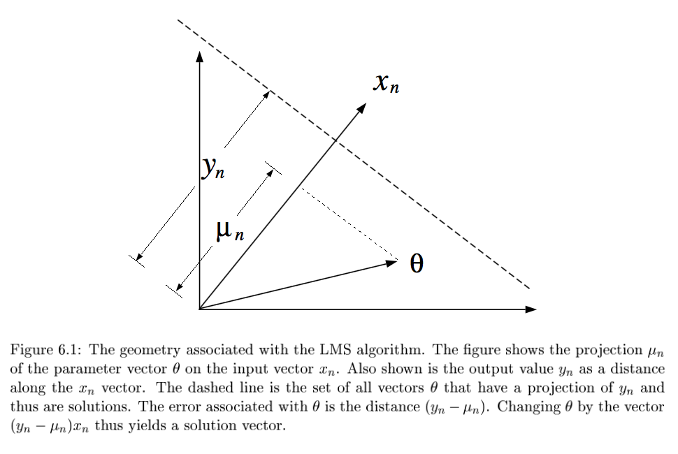
$y_n = \theta^T x_n + \epsilon_n$

$\theta^{(t+1)}=\theta^{(t)} + \alpha (y_n - \theta^{(t)T} x_n) x_n$

converges if $0 < \alpha < 2/

x_n

^2$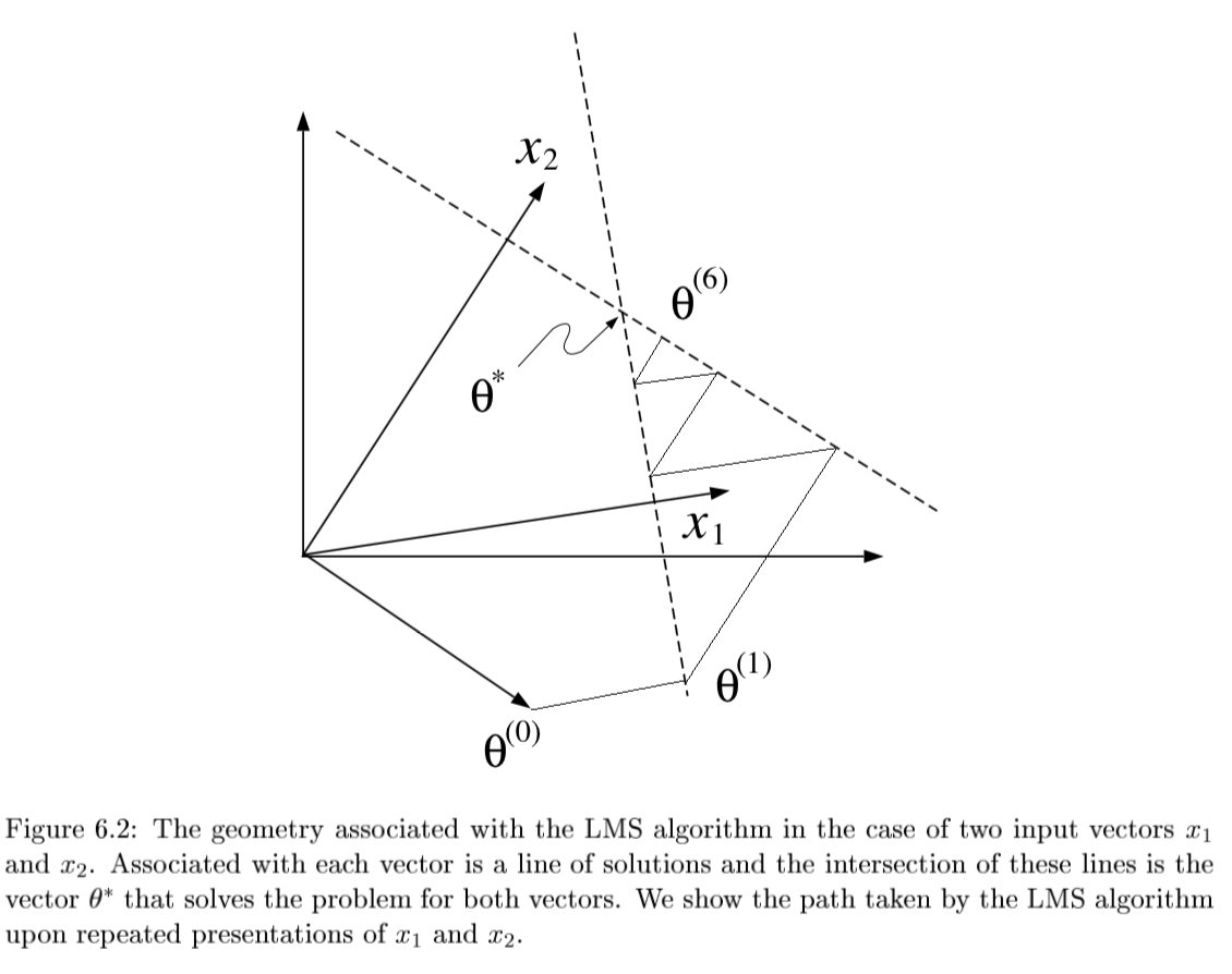

if N=p and all $x^{(i)}$ are lin. indepedent, then there exists exact solution $\theta$

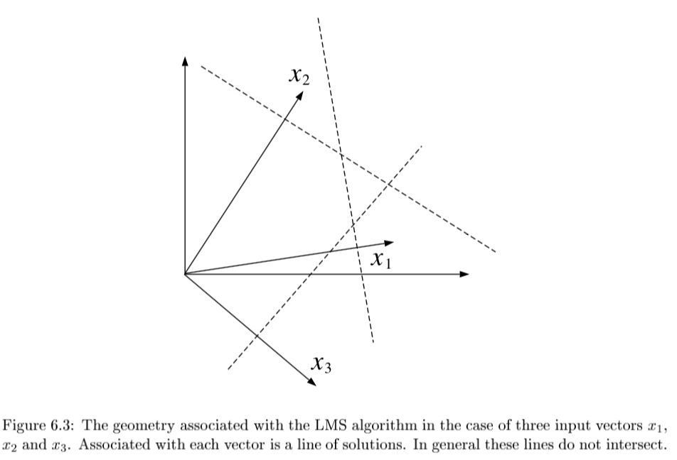
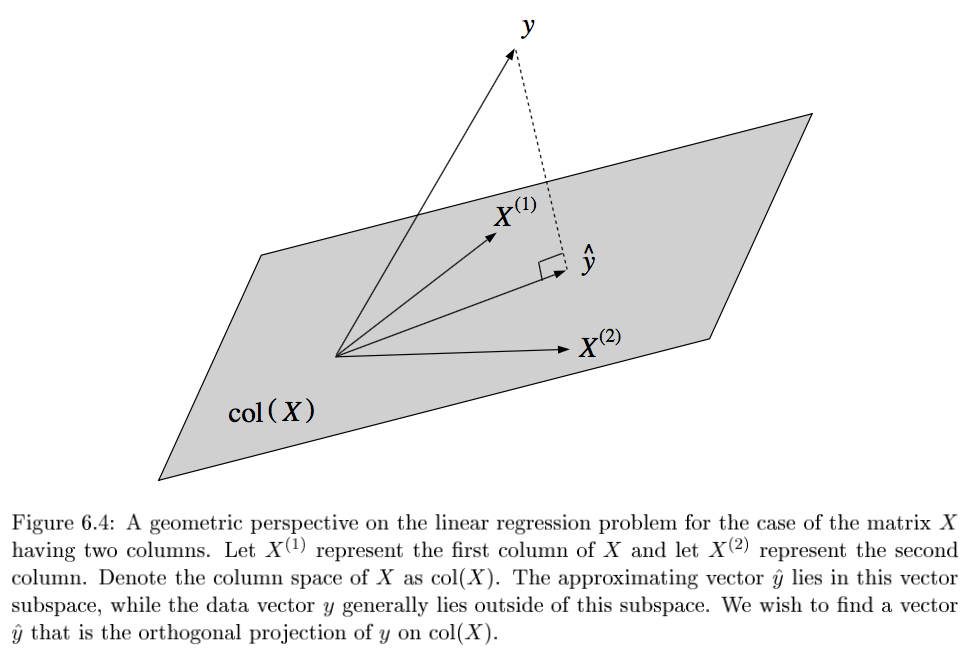
solving requires finding orthogonal projection of y on column space of X (n-dimensional geometries)
1. 3 Pfs
  1. geometry - $y-X\theta^*$ must be orthogonal to columns of X: $X^T(y-X\theta)=0$
  2. minimize least square cost function and differentiate
  3. show HY projects Y onto col(X)
- either of these approaches yield the normal eqns: $X^TX \theta^* = X^Ty$
SGD
- SGD converges to normal eqn
convergence analysis: requires $0 < \rho < 2/\lambda_{max} [X^TX]$
- algebraic analysis: expand $\theta^{(t+1)}$ and take $t \to \infty$
- geometric convergence analysis: consider contours of loss function
weighted least squares: $J(\theta)=\frac{1}{2}\sum_n w_n (y_n - \theta^T x_n)^2$
- yields $X^T WX \theta^* = X^T Wy$
probabilistic interpretation
- $p(y|x, \theta) = \frac{1}{(2\pi\sigma^2)^{N/2}} exp \left( \frac{-1}{2\sigma^2} \sum_{n=1}^N (y_n - \theta^T x_n)^2 \right)$
- $l(\theta; x,y) = - \frac{1}{2\sigma^2} \sum_{n=1}^N (y_n - \theta^T x_n)^2$
  - log-likelihood is equivalent to least-squares cost function

likelihood calcs

normal equation

$L(\theta) = \frac{1}{2} \sum_{i=1}^n (\hat{y}_i-y_i)^2$
$L(\theta) = 1/2 (X \theta - y)^T (X \theta -y)$
$L(\theta) = 1/2 (\theta^T X^T - y^T) (X \theta -y)$
$L(\theta) = 1/2 (\theta^T X^T X \theta - 2 \theta^T X^T y +y^T y)$
$0=\frac{\partial L}{\partial \theta} = 2X^TX\theta - 2X^T y$
$\theta = (X^TX)^{-1} X^Ty$

ridge regression

$L(\theta) = \sum_{i=1}^n (\hat{y}_i-y_i)^2+ \lambda \vert \vert \theta\vert \vert _2^2$
$L(\theta) = (X \theta - y)^T (X \theta -y)+ \lambda \theta^T \theta$
$L(\theta) = \theta^T X^T X \theta - 2 \theta^T X^T y +y^T y + \lambda \theta^T \theta$
$0=\frac{\partial L}{\partial \theta} = 2X^TX\theta - 2X^T y+2\lambda \theta$
$\theta = (X^TX+\lambda I)^{-1} X^T y$