![]()
FIGS: Fast Interpretable Greedy-Tree Sums
Yan Shuo Tan*, Chandan Singh*, Keyan Nasseri*, Abhineet Agarwal*, James Duncan, Omer Ronen, Matthew Epland, Aaron Kornblith, Bin Yu
Modern machine learning has achieved impressive prediction performance, but often sacrifices interpretability, a critical consideration in many problems. Here, we propose Fast Interpretable Greedy-Tree Sums (FIGS), an algorithm for fitting concise rule-based models. Specifically, FIGS generalizes the CART algorithm to work on sums of trees, growing a flexible number of them simultaneously. The total number of splits across all the trees is restricted by a pre-specified threshold, which ensures that FIGS remains interpretable. Extensive experiments show that FIGS achieves state-of-the-art performance across a wide array of real-world datasets when restricted to very few splits (e.g. less than 20). Theoretical and simulation results suggest that FIGS overcomes a key weakness of single-tree models by disentangling additive components of generative additive models, thereby significantly improving convergence rates for l2 generalization error. We further characterize the success of FIGS by quantifying how it reduces repeated splits, which can lead to redundancy in single-tree models such as CART. All code and models are released in a full-fledged package available on Github.
How does FIGS work?
Intuitively, FIGS works by extending CART, a typical greedy algorithm for growing a decision tree, to consider growing a sum of trees simultaneously (see Fig 1). At each iteration, FIGS may grow any existing tree it has already started or start a new tree; it greedily selects whichever rule reduces the total unexplained variance (or an alternative splitting criterion) the most. To keep the trees in sync with one another, each tree is made to predict the residuals remaining after summing the predictions of all other trees.FIGS is intuitively similar to ensemble approaches such as gradient boosting / random forest, but importantly since all trees are grown to compete with each other the model can adapt more to the underlying structure in the data. The number of trees and size/shape of each tree emerge automatically from the data rather than being manually specified.
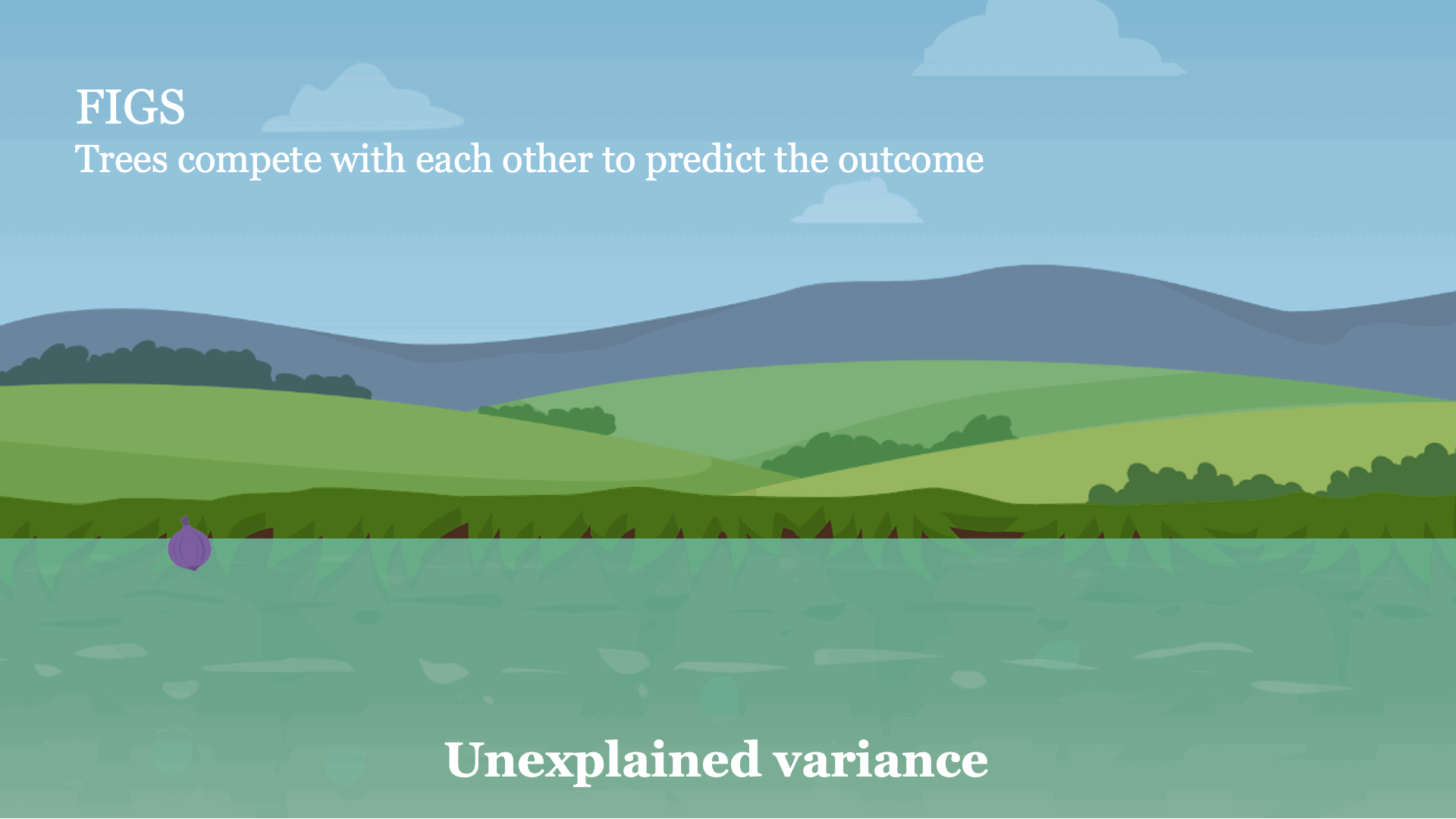
Fig 1. High-level intuition for how FIGS fits a model.
An example using FIGS
FIGS can be used in the same way as standard scikit-learn models: simply import a classifier or regressor and use thefit and predict methods. Here's a full example of
using it on a sample clinical dataset.
    from imodels import FIGSClassifier, get_clean_dataset
    from sklearn.model_selection import train_test_split

    # prepare data (in this a sample clinical dataset)
    X, y, feat_names = get_clean_dataset('csi_pecarn_pred')
    X_train, X_test, y_train, y_test = train_test_split(
    X, y, test_size=0.33, random_state=42)

    # fit the model
    model = FIGSClassifier(max_rules=4)  # initialize a model
    model.fit(X_train, y_train)   # fit model
    preds = model.predict(X_test) # discrete predictions: shape is (n_test, 1)
    preds_proba = model.predict_proba(X_test) # predicted probabilities: shape is (n_test, n_classes)

    # visualize the model
    model.plot(feature_names=feat_names, filename='out.svg', dpi=300)
This results in a simple model -- it contains only 4 splits (since we specified that the model
should have no more than 4 splits (max_rules=4). Predictions are made by summing the
value obtained from the appropriate leaf of each tree. This model is extremely interpretable, as a
physician can now (i) easily make predictions using the 4 relevant features and (ii) vet the model
to ensure it matches their domain expertise. Note that this model is just for illustration purposes,
and achieves ~84% accuracy.

Fig 2. Simple model learned by FIGS for predicting risk of cervical spinal injury.
model = FIGSClassifier()), resulting in a larger model (see Fig 3). Note
that the number of trees and how balanced they are emerges from the structure of the data -- only
the total number of rules may be specified.

Fig 3. Slightly larger model learned by FIGS for predicting risk of cervical spinal
injury.
Another example of using FIGS
Here, we examine the Diabetes classification dataset, in which eight risk factors were collected and used to predict the onset of diabetes within 5 five years. Fitting, several models we find that with very few rules, the model can achieve excellent test performance.
For example, Fig 2 shows a model fitted using the FIGS algorithm which achieves a test-AUC of 0.820 despite being extremely simple. In this model, each feature contributes independently of the others, and the final risks from each of three key features is summed to get a risk for the onset of diabetes (higher is higher risk). As opposed to a black-box model, this model is easy to interpret, fast to compute with, and allows us to vet the features being used for decision-making.

Fig 2. Simple model learned by FIGS for diabetes risk prediction.