Explaining text data by bridging interpretable models and LLMs

Explaining data is the overaching goal of data-driven science, allowing us to discover and quantitatively test hypotheses. The pursuit of data-driven explanations has led to the development of many interpretable models that allow a user to understand data patterns, such as decision trees, rule lists, and sparse linear models. However, these models are often not suitable to the peculiarities of text data, which is generally sparse, high-dimensional, and full of complex interactions. In contrast, LLMs have displayed impressive proficiency at handling text data, but they are often considered black boxes. Here, let's look at some recent work on bridging the gap between interpretable models and LLMs.
Interpretable models
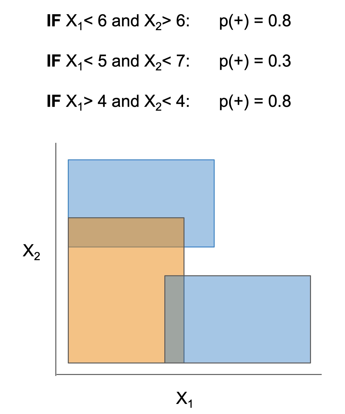
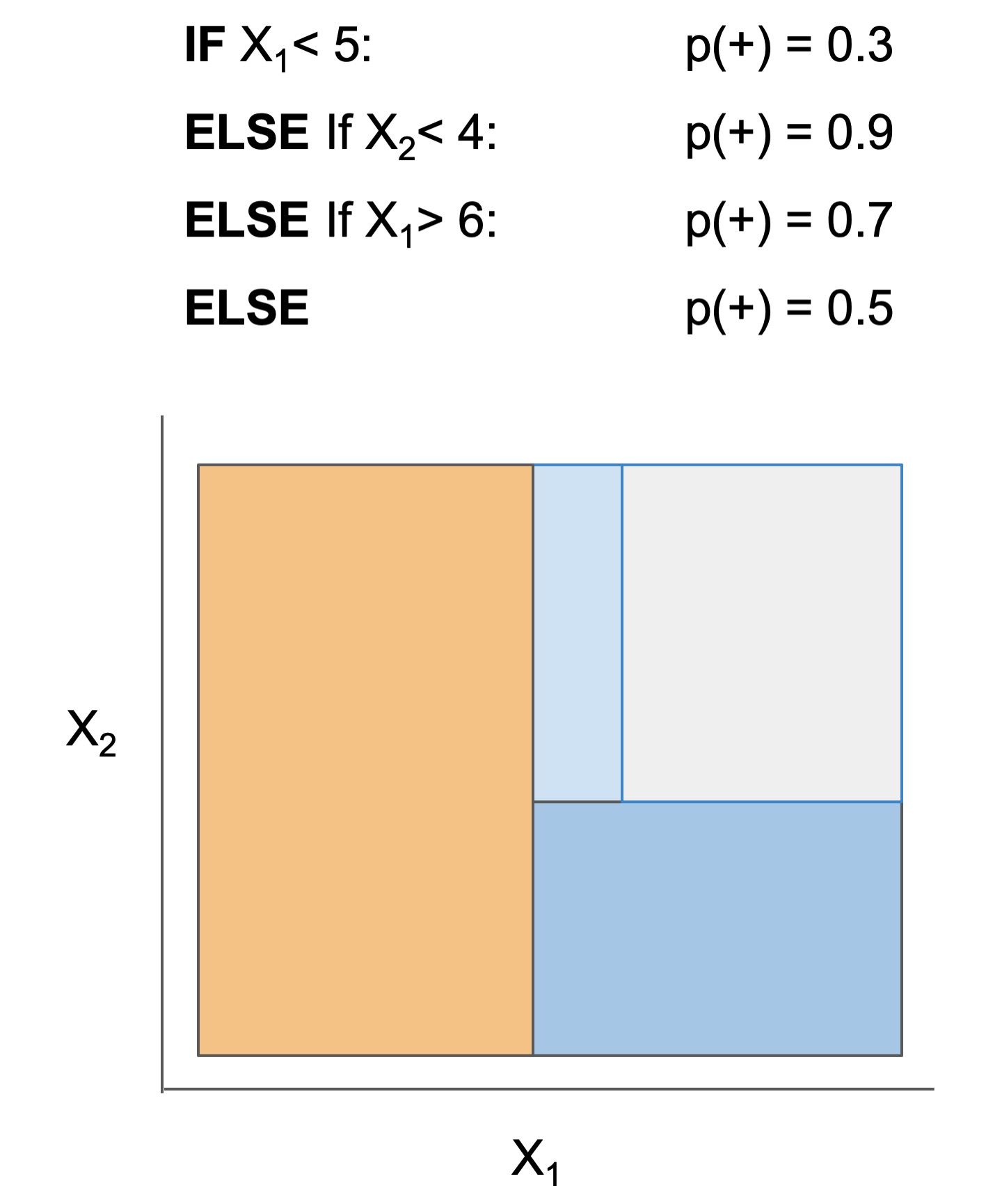
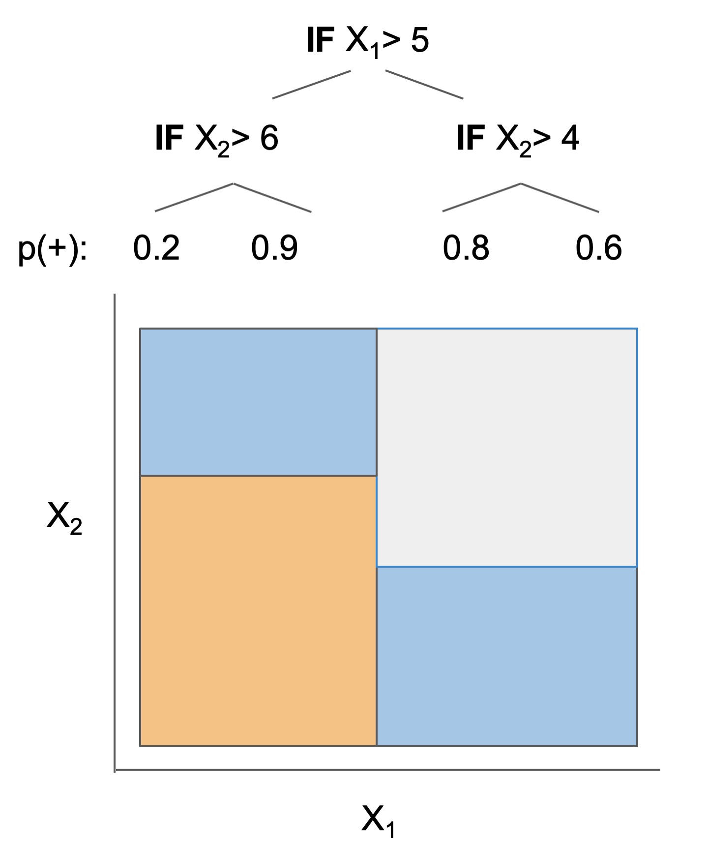
Many interpretable models have been proposed to interpret data involved in prediction problems (e.g. classification or regression). They may take slightly different forms (see some in Fig 1), but provide a complete description of the prediction process (as long as they're sufficiently accurate and small!). These models excel at tabular data, but struggle with other structured domains, such as text data.
| Rule set | Rule list | Rule tree | Algebraic models |
|---|---|---|---|
 |
 |
 |
 |
Figure 1. Different types of interpretable models. See scikit-learn friendly implementations in the imodels package.
Adding LLMs to interpretable models
Fig 2 shows some newer model forms that seek data explanations using LLMs/ interpretable models. For text data, These models are often more accurate than their interpretable counterparts, but still provide a complete description of the prediction process.
In the most direct case, an LLM is fed data corresponding to 2 groups (binary classification) and prompted to directly produce a description of the difference between the groups (D3/D5). Alternatively, given a dataset and a pre-trained LLM, iPrompt searches for a natural-language prompt that works well to predict on the dataset, which serves as a description of the data. This is more general than D3, as it is not restricted to binary groups, but is also more computationally intensive, as finding a good prompt often requires iterative LLM calls. Either of these approaches can also be applied recursively (TreePrompt), resulting in a hierarchical natural-language description of the data. Alternatively, many LLM answers to different questions can be concatenated into an embedding (QA-Emb), potentially incorporating bayesian iteration (BC-LLM), which can then be used to train a fully interpretable model, e.g. a linear model.

Figure 2. Different types of interpretable models, with text-specific approaches in bold. See scikit-learn friendly implementations below.
In parallel to these methods, Aug-imodels use LLMs to improve fully interpretable models directly. For example, Aug-Linear uses an LLM to augment a linear model, resulting in a more accurate model that is still completely interpretable. This is done by using an LLM only during training time to generate a dictionary of coefficients that is then extremely efficient and interpretable at inference time, while still maintaining reasonably high prediction accuracy (see Fig 3).

Figure 3. Aug-Linear uses an LLM to augment a linear model, resulting in a more accurate model that is still completely interpretable. The LLM is only used during training to generate a dictionary of coefficients, which is then used for efficient and interpretable inference.
The key to many of these explanation methods is finding ways to evaluate hypotheses without groundtruth, e.g. testing on follow-up experiments, synthetic data, prior findings, held-out data, counterfactuals, or new LLMs. This line of research is still in its infancy -- there's a lot to be done in combining LLMs and interpretable models!
Code reference below
Explainable modeling/steering
| Model | Reference | Output | Description |
|---|---|---|---|
| Tree-Prompt | 🗂️, 🔗, 📄, 📖, | Explanation + Steering |
Generates a tree of prompts to steer an LLM (Official) |
| iPrompt | 🗂️, 🔗, 📄, 📖 | Explanation + Steering |
Generates a prompt that explains patterns in data (Official) |
| AutoPrompt | ㅤㅤ🗂️, 🔗, 📄 | Explanation + Steering |
Find a natural-language prompt using input-gradients |
| D3 | 🗂️, 🔗, 📄, 📖 | Explanation | Explain the difference between two distributions |
| SASC | ㅤㅤ🗂️, 🔗, 📄 | Explanation | Explain a black-box text module using an LLM (Official) |
| Aug-Linear | 🗂️, 🔗, 📄, 📖 | Linear model | Fit better linear model using an LLM to extract embeddings (Official) |
| Aug-Tree | 🗂️, 🔗, 📄, 📖 | Decision tree | Fit better decision tree using an LLM to expand features (Official) |
| QAEmb | 🗂️, 🔗, 📄, 📖 | Explainable embedding |
Generate interpretable embeddings by asking LLMs questions (Official) |
| KAN | 🗂️, 🔗, 📄, 📖 | Small network |
Fit 2-layer Kolmogorov-Arnold network |
📖Demo notebooks 🗂️ Doc 🔗 Reference code 📄 Research paper ⌛ We plan to support other interpretable algorithms like RLPrompt, CBMs, and NBDT. If you want to contribute an algorithm, feel free to open a PR 😄
General utilities
| Model | Reference |
|---|---|
| 🗂️ LLM wrapper | Easily call different LLMs |
| 🗂️ Dataset wrapper | Download minimially processed huggingface datasets |
| 🗂️ Bag of Ngrams | Learn a linear model of ngrams |
| 🗂️ Linear Finetune | Finetune a single linear layer on top of LLM embeddings |
Quickstart
Installation: pip install imodelsx (or, for more control, clone and install from source)
Demos: see the demo notebooks
Natural-language explanations
Tree-prompt
from imodelsx import TreePromptClassifier
import datasets
import numpy as np
from sklearn.tree import plot_tree
import matplotlib.pyplot as plt

# set up data
rng = np.random.default_rng(seed=42)
dset_train = datasets.load_dataset('rotten_tomatoes')['train']
dset_train = dset_train.select(rng.choice(
    len(dset_train), size=100, replace=False))
dset_val = datasets.load_dataset('rotten_tomatoes')['validation']
dset_val = dset_val.select(rng.choice(
    len(dset_val), size=100, replace=False))

# set up arguments
prompts = [
    "This movie is",
    " Positive or Negative? The movie was",
    " The sentiment of the movie was",
    " The plot of the movie was really",
    " The acting in the movie was",
]
verbalizer = {0: " Negative.", 1: " Positive."}
checkpoint = "gpt2"

# fit model
m = TreePromptClassifier(
    checkpoint=checkpoint,
    prompts=prompts,
    verbalizer=verbalizer,
    cache_prompt_features_dir=None,  # 'cache_prompt_features_dir/gp2',
)
m.fit(dset_train["text"], dset_train["label"])


# compute accuracy
preds = m.predict(dset_val['text'])
print('\nTree-Prompt acc (val) ->',
      np.mean(preds == dset_val['label']))  # -> 0.7

# compare to accuracy for individual prompts
for i, prompt in enumerate(prompts):
    print(i, prompt, '->', m.prompt_accs_[i])  # -> 0.65, 0.5, 0.5, 0.56, 0.51

# visualize decision tree
plot_tree(
    m.clf_,
    fontsize=10,
    feature_names=m.feature_names_,
    class_names=list(verbalizer.values()),
    filled=True,
)
plt.show()
iPrompt
from imodelsx import explain_dataset_iprompt, get_add_two_numbers_dataset

# get a simple dataset of adding two numbers
input_strings, output_strings = get_add_two_numbers_dataset(num_examples=100)
for i in range(5):
    print(repr(input_strings[i]), repr(output_strings[i]))

# explain the relationship between the inputs and outputs
# with a natural-language prompt string
prompts, metadata = explain_dataset_iprompt(
    input_strings=input_strings,
    output_strings=output_strings,
    checkpoint='EleutherAI/gpt-j-6B', # which language model to use
    num_learned_tokens=3, # how long of a prompt to learn
    n_shots=3, # shots per example
    n_epochs=15, # how many epochs to search
    verbose=0, # how much to print
    llm_float16=True, # whether to load the model in float_16
)
--------
prompts is a list of found natural-language prompt strings
D3 (DescribeDistributionalDifferences)
from imodelsx import explain_dataset_d3
hypotheses, hypothesis_scores = explain_dataset_d3(
    pos=positive_samples, # List[str] of positive examples
    neg=negative_samples, # another List[str]
    num_steps=100,
    num_folds=2,
    batch_size=64,
)
SASC
Here, we explain a module rather than a dataset
from imodelsx import explain_module_sasc
# a toy module that responds to the length of a string
mod = lambda str_list: np.array([len(s) for s in str_list])

# a toy dataset where the longest strings are animals
text_str_list = ["red", "blue", "x", "1", "2", "hippopotamus", "elephant", "rhinoceros"]
explanation_dict = explain_module_sasc(
    text_str_list,
    mod,
    ngrams=1,
)
Aug-imodels
Use these just a like a scikit-learn model. During training, they fit better features via LLMs, but at test-time they are extremely fast and completely transparent.
from imodelsx import AugLinearClassifier, AugTreeClassifier, AugLinearRegressor, AugTreeRegressor
import datasets
import numpy as np

# set up data
dset = datasets.load_dataset('rotten_tomatoes')['train']
dset = dset.select(np.random.choice(len(dset), size=300, replace=False))
dset_val = datasets.load_dataset('rotten_tomatoes')['validation']
dset_val = dset_val.select(np.random.choice(len(dset_val), size=300, replace=False))

# fit model
m = AugLinearClassifier(
    checkpoint='textattack/distilbert-base-uncased-rotten-tomatoes',
    ngrams=2, # use bigrams
)
m.fit(dset['text'], dset['label'])

# predict
preds = m.predict(dset_val['text'])
print('acc_val', np.mean(preds == dset_val['label']))

# interpret
print('Total ngram coefficients: ', len(m.coefs_dict_))
print('Most positive ngrams')
for k, v in sorted(m.coefs_dict_.items(), key=lambda item: item[1], reverse=True)[:8]:
    print('\t', k, round(v, 2))
print('Most negative ngrams')
for k, v in sorted(m.coefs_dict_.items(), key=lambda item: item[1])[:8]:
    print('\t', k, round(v, 2))
KAN
import imodelsx
from sklearn.datasets import make_classification, make_regression
from sklearn.metrics import accuracy_score
import numpy as np

X, y = make_classification(n_samples=5000, n_features=5, n_informative=3)
model = imodelsx.KANClassifier(hidden_layer_size=64, device='cpu',
                               regularize_activation=1.0, regularize_entropy=1.0)
model.fit(X, y)
y_pred = model.predict(X)
print('Test acc', accuracy_score(y, y_pred))

# now try regression
X, y = make_regression(n_samples=5000, n_features=5, n_informative=3)
model = imodelsx.kan.KANRegressor(hidden_layer_size=64, device='cpu',
                                  regularize_activation=1.0, regularize_entropy=1.0)
model.fit(X, y)
y_pred = model.predict(X)
print('Test correlation', np.corrcoef(y, y_pred.flatten())[0, 1])
General utilities
Easy baselines
Easy-to-fit baselines that follow the sklearn API.
from imodelsx import LinearFinetuneClassifier, LinearNgramClassifier
# fit a simple one-layer finetune on top of LLM embeddings
m = LinearFinetuneClassifier(
    checkpoint='distilbert-base-uncased',
)
m.fit(dset['text'], dset['label'])
preds = m.predict(dset_val['text'])
acc = (preds == dset_val['label']).mean()
print('validation acc', acc)
LLM wrapper
Easy API for calling different language models with caching (much more lightweight than langchain).
import imodelsx.llm
# supports any huggingface checkpoint or openai checkpoint (including chat models)
llm = imodelsx.llm.get_llm(
    checkpoint="gpt2-xl",  # text-davinci-003, gpt-3.5-turbo, ...
    CACHE_DIR=".cache",
)
out = llm("May the Force be")
llm("May the Force be") # when computing the same string again, uses the cache
Data wrapper
API for loading huggingface datasets with basic preprocessing.
import imodelsx.data
dset, dataset_key_text = imodelsx.data.load_huggingface_dataset('ag_news')
# Ensures that dset has a split named 'train' and 'validation',
# and that the input data is contained for each split in a column given by {dataset_key_text}
Related work
- imodels package (JOSS 2021 github) - interpretable ML package for concise, transparent, and accurate predictive modeling (sklearn-compatible).
- Rethinking Interpretability in the Era of Large Language Models (arXiv 2024 pdf) - overview of using LLMs to interpret datasets and yield natural-language explanations
- Experiments in using clinical rule development: github
- Experiments in automatically generating brain explanations: github
- Interpretation regularization (ICML 2020 pdf, github) - penalizes CD / ACD scores during training to make models generalize better
Sub-modules
imodelsx.auglinearimodelsx.augtreeimodelsx.cache_save_utilsimodelsx.d3imodelsx.dataimodelsx.embeddingsimodelsx.ipromptimodelsx.kanimodelsx.linear_finetune-
Simple scikit-learn interface for finetuning a single linear layer on top of LLM embeddings.
imodelsx.linear_ngram-
Simple scikit-learn interface for finetuning a single linear layer on top of LLM embeddings.
imodelsx.llmimodelsx.metricsimodelsx.process_resultsimodelsx.qaembimodelsx.sascimodelsx.submit_utilsimodelsx.treepromptimodelsx.utilimodelsx.viz