Deep Learning view markdown
This note covers miscellaneous deep learning, with an emphasis on different architectures + empirical tricks.
See also notes in 📌 unsupervised learning, 📌 disentanglement, 📌 nlp, 📌 transformers
historical top-performing nets
- LeNet (1998)
- first, used on MNIST
- AlexNet (2012)
- landmark (5 conv layers, some pooling/dropout)
- ZFNet (2013)
- fine tuning and deconvnet
- VGGNet (2014)
- 19 layers, all 3x3 conv layers and 2x2 maxpooling
- GoogLeNet (2015)
- lots of parallel elements (called Inception module)
- Msft ResNet (2015)
- very deep - 152 layers
- connections straight from initial layers to end
- only learn “residual” from top to bottom
- very deep - 152 layers
- Region Based CNNs (R-CNN - 2013, Fast R-CNN - 2015, Faster R-CNN - 2015)
- object detection
- Generating image descriptions (Karpathy , 2014)
- RNN+CNN
- Spatial transformer networks (2015)
- transformations within the network
- Segnet (2015)
- encoder-decoder network
- Unet (Ronneberger, 2015)
- applies to biomedical segmentation
- Pixelnet (2017) - predicts pixel-level for different tasks with the same architecture - convolutional layers then 3 FC layers which use outputs from all convolutional layers together
- Squeezenet
- Yolonet
- Wavenet
- Densenet
- NASNET
- Efficientnet (2019)
basics
- basic perceptron update rule
- if output is 0, label is 1: increase active weights
- if output is 1, label is 0: decrease active weights
- perceptron convergence thm - if data is linearly separable, perceptron learning algorithm wiil converge
- transfer / activation functions
- sigmoid(z) = $\frac{1}{1+e^{-x}} = \frac{e^x}{e^x+1}$
- Binary step
- TanH (preferred to sigmoid)
- Rectifier = ReLU
- Leaky ReLU - still has some negative slope when <0
- rectifying in electronics converts analog -> digital
- rare to mix and match neuron types
- deep - more than 1 hidden layer
- mean-squared error (regression loss) = $\frac{1}{2}(y-\hat{y})^2$
- cross-entropy loss (classification loss) = $=-\sum_j y_j \ln \hat{p}_j$
- for binary classification, $y_j$ would take on 0 or 1 and $\hat y_j$ would be a probability
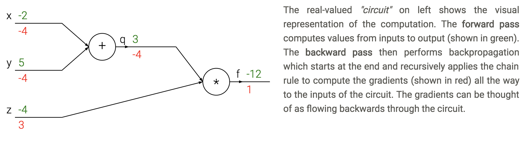
- backpropagation - application of reverse mode automatic differentiation to neural networks’s loss
- apply the chain rule from the end of the program back towards the beginning
- $\frac{dL}{d \theta_i} = \frac{dL}{dz} \frac{\partial z}{\partial \theta_i}$
- sum $\frac{dL}{dz}$ if neuron has multiple outputs z
- L is output
- $\frac{\partial z}{\partial \theta_i}$ is actually a Jacobian (deriv each $z_i$ wrt each $\theta_i$ - these are vectors)
- each gate usually has some sparsity structure so you don’t compute whole Jacobian
- apply the chain rule from the end of the program back towards the beginning
- pipeline
- initialize weights, and final derivative ($\frac{dL}{dL}=1$)
- for each batch
- run network forward to compute outputs at each step
- compute gradients at each gate with backprop
- update weights with SGD
training
- vanishing gradients problem - neurons in earlier layers learn more slowly than in later layers
- happens with sigmoids
- dead ReLus
- exploding gradients problem - gradients are significantly larger in earlier layers than later layers
- RNNs
- batch normalization - whiten inputs to all neurons (zero mean, variance of 1)
- do this for each input to the next layer
- dropout - randomly zero outputs of p fraction of the neurons during training
- like learning large ensemble of models that share weights
- 2 ways to compensate (pick one)
- at test time multiply all neurons’ outputs by p
- during training divide all neurons’ outputs by p
- softmax - takes vector z and returns vector of the same length
- makes it so output sums to 1 (like probabilities of classes)
- tricks to squeeze out performance
- ensemble models
- (stochastic) weight averaging can help a lot
- test-time augmentation
- this could just be averaging over dropout resamples as well
- gradient checkpointing (2016 paper)
- 10x larger DNNs into memory with 20% increase in comp. time
- save gradients for a carefully chosen layer to let you easily recompute
CNNs
- kernel here means filter
- convolution G- takes a windowed average of an image F with a filter H where the filter is flipped horizontally and vertically before being applied
- G = H $\ast$ F
- if we do a filter with just a 1 in the middle, we get the exact same image
- you can basically always pad with zeros as long as you keep 1 in middle
- can use these to detect edges with small convolutions
- can do Guassian filters
- 1st-layer convolution typically sum over all color channels
- 1x1 conv - still convolves over channels
- pooling - usually max - doesn’t pool over depth
- people trying to move away from this - larger strides in conversation layers
- stacking small layers is generally better
- most of memory impact is usually from activations from each layer kept around for backdrop
- visualizations
- layer activations (maybe average over channels)
- visualize the weights (maybe average over channels)v
- feed a bunch of images and keep track of which activate a neuron most
- t-SNE embedding of images
- occluding
- weight matrices have special structure (Toeplitz or block Toeplitz)
- input layer is usually centered (subtract mean over training set)
- usually crop to fixed size (square input)
- receptive field - input region
- stride m - compute only every mth pixel
- downsampling
- max pooling - backprop error back to neuron w/ max value
- average pooling - backprop splits error equally among input neurons
- data augmentation - random rotations, flips, shifts, recolorings
- siamese networks - extract features twice with same net then put layer on top
- ex. find how similar to representations are
RNNs
- feedforward NNs have no memory so we introduce recurrent NNs
- able to have memory
- truncated - limit number of times you unfold
- $state_{new} = f(state_{old},input_t)$
- ex. $h_t = tanh(W h_{t-1}+W_2 x_t)$
- train with backpropagation through time (unfold through time)
- truncated backprop through time - only run every k time steps
- error gradients vanish exponentially quickly with time lag
- LSTMS
- have gates for forgetting, input, output
- easy to let hidden state flow through time, unchanged
- gate $\sigma$ - pointwise multiplication
- multiply by 0 - let nothing through
- multiply by 1 - let everything through
- forget gate - conditionally discard previously remembered info
- input gate - conditionally remember new info
- output gate - conditionally output a relevant part of memory
- GRUs - similar, merge input / forget units into a single update unit
graph neural networks
- Theoretical Foundations of Graph Neural Networks
- inputs are graphs
- e.g. molecule input to classification
- one big study: a deep learning appraoch to antibiotic discovery (stokes et al. 2020) - using GNN classification of antibiotic resistance, came up with 100 candidate antibiotics and were able to test them
- e.g. traffic maps - nodes are intersections
- invariances in CNNs: translational, neighbor pixels relate a lot more
- simplest setup: no edges, each node $i$ has a feature vector $x_i$ (really a set not a graph)
- X is a matrix where each row is a feature vector
- note that permuting rows of X shouldn’t change anything
- permutation invariant: $f(PX) = f(X)$ for all permutation matrices $P$
- e.g. $\mathbf{P}{(2,4,1,3)} \mathbf{X}=\left[\begin{array}{llll}0 & 1 & 0 & 0 \ 0 & 0 & 0 & 1 \ 1 & 0 & 0 & 0 \ 0 & 0 & 1 & 0\end{array}\right]\left[\begin{array}{lll}- & \mathbf{x}{1} & - \ - & \mathbf{x}{2} & - \ - & \mathbf{x}{3} & - \ - & \mathbf{x}{4} & -\end{array}\right]=\left[\begin{array}{lll}- & \mathbf{x}{2} & - \ - & \mathbf{x}{4} & - \ - & \mathbf{x}{1} & - \ - & \mathbf{x}_{3} & -\end{array}\right]$
- ex. Deep Sets model (zaheer et al. ‘17): $f(X) = \phi \left (\sum_k \psi(x_i) \right)$
- permutation equivariant: $f(PX) = P f(X)$ - useful for when we want answers at the node level
- graph: augment set of nodes with edges between them (store as an adjacency matrix)
- permuting permutation matrix to A requires operating on both rows and cols: $PAP^T$
- permutation invariance: $ f\left(\mathbf{P X}, \mathbf{P A P}^{\top}\right)=f(\mathbf{X}, \mathbf{A})$
- permutation equivariance: $f\left(\mathbf{P X}, \mathbf{P A P}^{\top}\right)=\mathbf{P} f(\mathbf{X}, \mathbf{A})$
- can now write an equivariant function that extracts features not only of X, but also its neighbors: $g(x_b, X_{\mathcal N_b})$
- tasks: node classification, graph classification, link (edge) prediction)
- 3 flavors of GNN layers for extracting features from nodes / neighbors: simplest to most complex
- message-passing actually passes vectors to be sent across edges
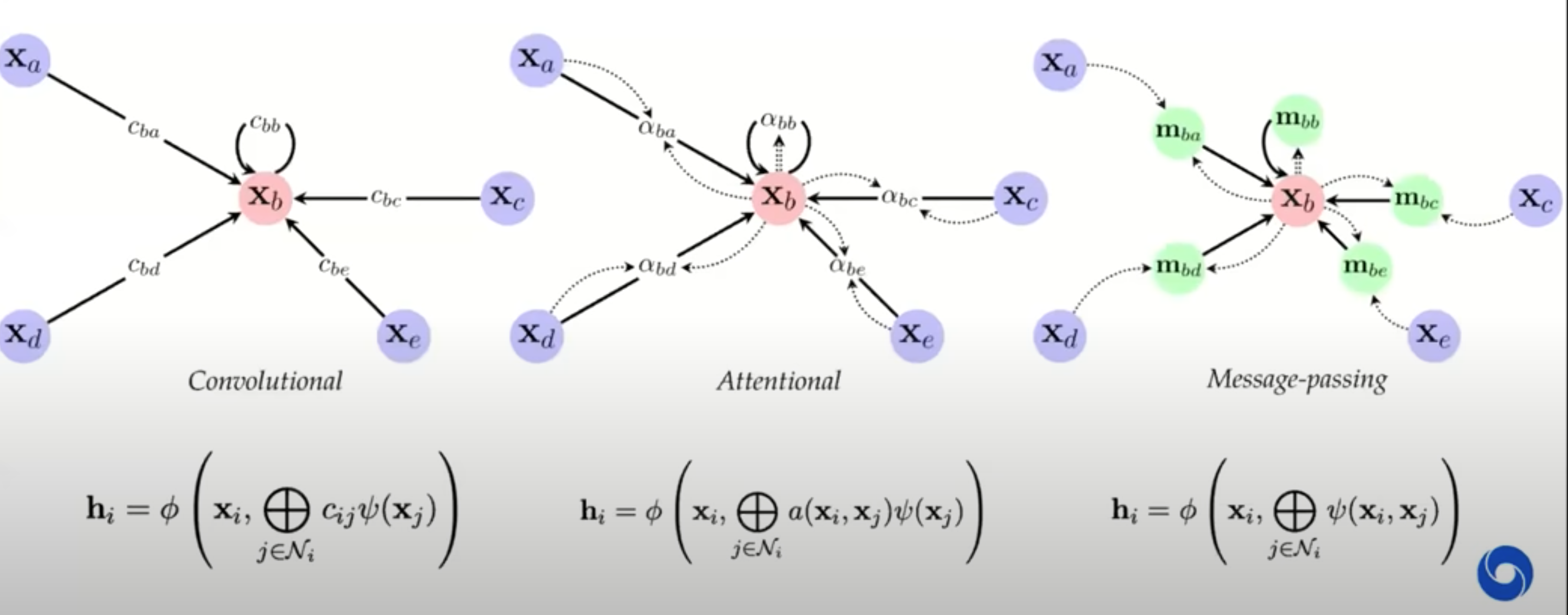
- previous approaches map on to gnns well
- GNNs explicitly construct local features, much like previous works
- local objectives: features of nodes i and j should predict existence of edge $(i, j)$
- random-walk objectives: features should be similar if i and j co-occur on a short random walk (e.g. deepwalk, node2vec, line)
- similarities to NLP if we think of words as nodes and sentences as walks
- we can think of transformers as fully-connect graph networks with attentional form of GNN layers
- one big difference: positional embeddings often used, making the input not clearly a graph
- these postitional embeddings often take the form of sin/cos - very similar to DFT eigenvectors of a graph
- one big difference: positional embeddings often used, making the input not clearly a graph
- we can think of transformers as fully-connect graph networks with attentional form of GNN layers
- spectral gnns
- operate on graph laplacian matrix $L = D - A$ where $D$ is degree matrix and $A$ is adjacency matrix - more mathematically convenient
- probabilistic modeling - e.g. assome markov random field and try to learn parameters
- this connects well to a message-passing GNN
- GNNs explicitly construct local features, much like previous works
- GNN limitations
- ex. can we tell whether 2 graphs are isomorphic - often no?
- can make GNNs more powerful by adding positional features, etc.
- can also embed sugraphs together
- continuous case is more difficult
- geometric deep learning: invariances and equivariances can be applied generally to get a large calss of architectures between convolutions and graphs
misc architectural components
- coordconv - break translation equivariance by passing in i, j coords as extra filters
- deconvolution = transposed convolution = fractionally-strided convolution - like upsampling
top-down feedback
- Look and Think Twice: Capturing Top-Down Visual Attention With Feedback Convolutional Neural Networks (2015)
- neurons in the feedback hidden layers update their activation status to maximize the confidence output of the target top neuron
-
[Top-Down Neural Attention by Excitation Backprop SpringerLink](https://link.springer.com/article/10.1007/s11263-017-1059-x) (2017) - top-down attention maps by extending winner-take-all (WTA) to probabilistic maps
- Modeling visual attention via selective tuning - ScienceDirect (1995)
- original WTA paper provides only binary maps
- Bottom-Up and Top-Down Reasoning with Hierarchical Rectified Gaussians (2016)
- Beyond Skip Connections: Top-Down Modulation for Object Detection (shrivastava…malik, gupta, 2017)
- Learning to Combine Top-Down and Bottom-Up Signals in Recurrent Neural Networks with Attention over Modules (mittal…bengio, 2020)
- Very similar — each layer passes attention (1) to next layer (2) to itself (3) to previous layer
- Fast and Slow Learning of Recurrent Independent Mechanisms (madan…bengio, 2021)
- Inductive Biases for Deep Learning of Higher-Level Cognition (goyal & bengio, 2021)
- Neural Networks with Recurrent Generative Feedback (huang…tsao, anandkumar, 2020)
- Deconvolutional Generative Model DGM - hierarchical latent variables capture variation in images + generate images from a coarse to fine detail using deconvolution operations
- A generative vision model that trains with high data efficiency and breaks text-based CAPTCHAs (vicarious, 2016)
- bayesian model + crf on latents breaks captchas
- Combining Top-Down and Bottom-Up Segmentation (2008) (pre-DNNs)
- Bottom-up segmentation: group chunks of image into ever-larger regions based on e.g. texture similarity
- Top-down segmentation: find object boundaries based on label info
- Perceiver: General Perception with Iterative Attention (2021)
- Integration of top-down and bottom-up visual processing using a recurrent convolutional–deconvolutional neural network for semantic segmentation (2019)
- Very similar to our idea - they have deconvolved feedback to earlier layers
- Architecture’s weird, tho - feedback only goes back a few layers
- Extremely applied - their result is “we beat SOTA by 3%”
- Attentional Neural Network: Feature Selection Using Cognitive Feedback (2014)
- Efficient Learning of Deep Boltzmann Machines (2010)
neural architecture search (NAS)
- One Network Doesn’t Rule Them All: Moving Beyond Handcrafted Architectures in Self-Supervised Learning (girish, dey et al. 2022) - use NAS for self-supervised setting rather than supervised
- A Deeper Look at Zero-Cost Proxies for Lightweight NAS · The ICLR Blog Track (white…bubeck, dey, 2022)
- tl;dr A single minibatch of data is used to score neural networks for NAS instead of performing full training.
misc
- Deep Learning Interviews: Hundreds of fully solved job interview questions from a wide range of key topics in AI
- adaptive pooling can help deal with different sizes
- NeRF: Representing Scenes as Neural Radiance Fields for View Synthesis
- given multiple views, generate depth map + continuous volumetric repr.
- dnn is overfit to only one scene
- inputs: a position and viewing direction
- output: for that position, density (is there smth at this location) + color (if there is smth at this location)
- then, given new location / angle, send a ray through for each pixel and see color when it hits smth
- Implicit Neural Representations with Periodic Activation Functions
- similar paper
- optimal brain damage - starts with fully connected and weeds out connections (Lecun)
- tiling - train networks on the error of previous networks
- Language model compression with weighted low-rank factorization (hsu et al. 2022) - incorporate fisher info of weights when compressing via SVD (this helps preserve the weights which are important for prediction)
- can represent a full-rank weight matrix as a product of low-rank matrices, e.g. to get rank r repr of 10x10 matrix, make it a product of a 10xr and an rx10 matrix
- people often use SVD to posthoc compress a DNN
empirical notes
nrom layers
Batch Normalization - for a mini-batch $\mathcal{B} = {x_1, x_2, \ldots, x_m}$, normalize each feature across the batch dimension:
[\mu_\mathcal{B} = \frac{1}{m} \sum_{i=1}^{m} x_i]
[\sigma_\mathcal{B}^2 = \frac{1}{m} \sum_{i=1}^{m} (x_i - \mu_\mathcal{B})^2]
[\hat{x}i = \frac{x_i - \mu*\mathcal{B}}{\sqrt{\sigma\mathcal{B}^2 + \epsilon}}, \quad y_i = \gamma \hat{x}_i + \beta]
where $\gamma$ and $\beta$ are learnable scale and shift parameters, and $\epsilon$ is a small constant for numerical stability.
Layer Normalization - same thing except normalize across features (don’t average over tokens):
[\mu = \frac{1}{d} \sum_{i=1}^{d} x_i]
[\sigma^2 = \frac{1}{d} \sum_{i=1}^{d} (x_i - \mu)^2]
[\hat{x}_i = \frac{x_i - \mu}{\sqrt{\sigma^2 + \epsilon}}, \quad y_i = \gamma_i \hat{x}_i + \beta_i]
where $\gamma, \beta \in \mathbb{R}^d$ are learnable per-feature parameters.
RMS Normalization
Root Mean Square normalization drops the mean-centering step:
[\text{RMS}(x) = \sqrt{\frac{1}{d} \sum_{i=1}^{d} x_i^2}]
[\hat{x}_i = \frac{x_i}{\sqrt{\text{RMS}(x)^2 + \epsilon}} \quad y_i = \gamma_i \hat{x}_i]
where $\gamma \in \mathbb{R}^d$ is a learnable scale parameter. Note there is no shift parameter $\beta$, and no mean subtraction — making it cheaper to compute than LayerNorm