
FastSmallTree: Implementing compact, fast decision trees via Autoresearch
Chandan Singh · September 2026
Standard decision trees are fit greedily, so they end up larger than they need to be and harder to interpret. Optimal-tree solvers such as GOSDT and STreeD instead find the tree that provably minimizes error plus a penalty per leaf, but they are slow. Using autoresearch, we build FastSmallTree, an implementation that achieves useful speedups on real-world problems for fitting small trees (mostly by effectively compiling things into numba). On held-out benchmarks, it maintains the accuracy of existing optimal tree packages while sometimes providing significant speedups, sometimes >20×.
1. Quickstart & example usage
from imodels import FastSmallTreeClassifier
from sklearn.datasets import load_breast_cancer
from sklearn.model_selection import train_test_split

X, y = load_breast_cancer(return_X_y=True, as_frame=True)
X_train, X_test, y_train, y_test = train_test_split(X, y, random_state=42)

model = FastSmallTreeClassifier(regularization=0.05).fit(X_train, y_train)
preds = model.predict(X_test)
regularization is the only hyperparameter: larger values give smaller trees. The fitted model reports whether the search finished, and what it proved:
model.optimal_      # True: no other tree on these features scores better
model.objective_    # 0.1775, the proven minimum of error + 0.05 * leaves
model.n_leaves_     # 2
print(model)        # the tree, as nested if/else on the caller's feature names
Visualize the tree
The certified tree is stored as an ordinary sklearn DecisionTreeClassifier in
model.estimator_, so it works with sklearn-compatible libraries (plot_tree,
export_text, feature_importances_), e.g. dtreeviz:
import dtreeviz  # pip install dtreeviz

model = FastSmallTreeClassifier(
    regularization=0.03)
model.fit(X_train, y_train)

viz = dtreeviz.model(
    model.estimator_, X_train, y_train,
    feature_names=X.columns,
    target_name="diagnosis",
    class_names=["malignant", "benign"])
viz.view()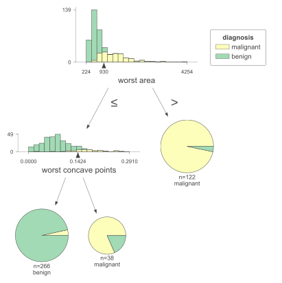
regularization=0.03 on the breast cancer
training split. Thresholds sit midway between neighbouring training values, as in sklearn.2. Experimental results
FastSmallTree was produced by the autoresearch loop of
Agentic-imodels (code on
github): an agent was given a working
exact solver, a fixed benchmark, and a rule that no change may return a non-optimal tree.
It then proposed, proved and measured new bounds, keeping those that yielded speed ups on the visible set of problems.
The visible set consists of 70 problems (14 datasets × 5 values of regularization),
each with a 30-second time limit and 6-GB memory limit.
The 14 visible datasets (from the GOSDT repo)
| dataset | what it is | rows | features | binary splits | classes |
|---|---|---|---|---|---|
chudi | Two-feature example from the GOSDT experiments | 77 | 2 | 46 | 2 |
monk_3 | UCI MONK's problem 3, one-hot | 122 | 11 | 11 | 2 |
monk_1 | UCI MONK's problem 1, one-hot | 124 | 11 | 11 | 2 |
iris | UCI Iris | 150 | 4 | 118 | 3 |
monk_2 | UCI MONK's problem 2, one-hot | 169 | 11 | 11 | 2 |
tic-tac-toe | UCI Tic-Tac-Toe endgames | 958 | 9 | 27 | 2 |
gaussian_1k | Synthetic, one continuous feature | 1,000 | 1 | 999 | 2 |
fico_1k | FICO HELOC credit, 1,000-row sample, raw features | 1,000 | 23 | 1,357 | 2 |
sine_1k | Synthetic, one continuous feature | 1,000 | 1 | 999 | 2 |
car_evaluation | UCI Car Evaluation, binarized | 1,728 | 15 | 15 | 2 |
coupon_bar | In-vehicle coupon recommendation, bar coupons | 1,913 | 14 | 14 | 2 |
compas_binned | ProPublica COMPAS recidivism, binarized | 6,907 | 12 | 12 | 2 |
fico_binary | FICO HELOC credit, binarized | 10,459 | 17 | 17 | 2 |
compas_processed | ProPublica COMPAS recidivism, processed | 12,381 | 22 | 621 | 2 |
All 14 come from the GOSDT reference repository, each run at five penalties per leaf (0.1, 0.05, 0.02, 0.01, 0.005): 70 problems. Binary splits is what the solver searches: one per binary feature and one per distinct value of a numeric one, which is why fico_1k and compas_processed hold the problems nobody certifies.
The 14 hidden datasets (from TabArena)
| stands in for | TabArena source | rows | features | binary splits | majority | classes |
|---|---|---|---|---|---|---|
chudi | blood-transfusion-service-center | 77 | 2 | 32 / 46 | 0.61 / 0.61 | 2 |
monk_3 | seismic-bumps | 122 | 11 | 11 / 11 | 0.51 / 0.51 | 2 |
monk_1 | Marketing_Campaign | 124 | 11 | 11 / 11 | 0.50 / 0.50 | 2 |
iris | maternal_health_risk | 150 | 4 | 83 / 118 | 0.33 / 0.33 | 3 |
monk_2 | Is-this-a-good-customer | 169 | 11 | 11 / 11 | 0.62 / 0.62 | 2 |
tic-tac-toe | qsar-biodeg | 958 | 9 | 27 / 27 | 0.65 / 0.65 | 2 |
gaussian_1k | credit-g | 1,000 | 1 | 920 / 999 | 0.70 / 0.70 | 2 |
fico_1k | polish_companies_bankruptcy | 1,000 | 23 | 1,357 / 1,357 | 0.59 / 0.54 | 2 |
sine_1k | Fitness_Club | 1,000 | 1 | 876 / 999 | 0.55 / 0.51 | 2 |
car_evaluation | Bioresponse | 1,728 | 15 | 15 / 15 | 0.70 / 0.70 | 2 |
coupon_bar | hazelnut-spread-contaminant-detection | 1,913 | 14 | 14 / 14 | 0.59 / 0.59 | 2 |
compas_binned | E-CommereShippingData | 6,907 | 12 | 12 / 12 | 0.54 / 0.54 | 2 |
fico_binary | HR_Analytics_Job_Change_of_Data_Scientists | 10,459 | 17 | 17 / 17 | 0.54 / 0.52 | 2 |
compas_processed | credit_card_clients_default | 12,381 | 22 | 625 / 621 | 0.69 / 0.69 | 2 |
Each development dataset has a stand-in drawn from a
TabArena classification dataset by a fixed rule (originals
largest first, each taking the smallest unused source with enough rows of each class). A
stand-in matches its original's rows and features exactly and its class balance within 0.05,
keeping the features with the most mutual information with the label; numeric features are
quantile-binned to match the original's number of binary splits, shown in gray. chudi and iris
fall short because their sources have too few distinct values. TabArena's HELOC and coupon
datasets are excluded, since the development suite already contains them. Builder, manifest
and per-problem results:
agentic-imodels,
baselines/benchmarks/external/.
Fig 1 plots the fitted loss (y-axis, lower is better) against the time per problem (x-axis, left is faster) for every version the loop produced against the baselines. We compare against four published baselines: GOSDT (Lin et al., 2020), its successor gosdt-guesses (McTavish et al., 2022), STreeD (van der Linden et al., 2023), and the near-optimal SPLIT (Babbar et al., 2025). Fig 1A shows the visible set while the other three panels evaluate on the hidden set in different ways. When a solver returns no tree for a problem, its criterion there is that of a single leaf predicting the majority class, and its time is the seconds it spent before stopping, capped at the panel's time limit (the full limit if it ran out of time, less if it stopped early at the 6 GB memory limit).
- Autoresearch versions, exact
- Autoresearch versions, approximate
- Baselines, exact
- Baselines, approximate
- FastSmallTree
Visible set (5 penalties, 30 s per problem)
Hidden set (5 penalties, 30 s per problem)
Hidden set, full size (penalty 0.05, 30 min per problem)
Hidden set (5 penalties, 4 h per problem, big Linux server)
Fig 1. Tree quality against speed. A: the visible set the autoresearch loop was scored on, 70 problems (14 datasets × 5 penalties) at 30 s each. This plot shows all the versions tried by the loop. B: the same 70-problem protocol on TabArena-14, held-out datasets never used during development. C: TabArena-14 at full size, every row and column kept, at one penalty (0.05) with 30 minutes a problem. D: TabArena-14's 70 problems with 4 hours a problem instead of 30 s, and the same 6 GB. A–C all evaluate using a MacBook Air M5, while D uses a Linux server (two Xeon Platinum 8468V, 88 cores). Each point is a solver's geometric mean, over a panel's problems, of the time spent (up to the cap) and of the criterion its tree scores, error plus penalty times leaves. Blue: versions whose every bound is admissible. Dark blue: versions that are approximate (non-optimal). Light and dark gray: baselines, exact and approximate. Large points average three runs.
Extra details on experimental settings
A. Every returned tree is re-scored from the raw data and checked against its problem's certified optimum, so a solver cannot score by misreporting. v46's points are from the fixed code; a draft certified two wrong trees here (Methods).
B. TabArena-14 has no certified optima, so a certificate there is checked against the best tree any run of any solver returned.
C. One run at a single penalty (0.05) on each of the 14 datasets, so the panel is read for the ordering rather than a close criterion race; several optima at that penalty are a single leaf, which every solver finds at once. Three kinds of baseline failure are charged as no tree: a stop at the 6 GB cap (GOSDT on 8 problems, SPLIT on 8), a run killed after twice its budget (STreeD on 2), and an operating-system kill for outgrowing memory (STreeD on coupon_bar, signal 9 after five minutes). GOSDT runs in a child process that the harness can stop at the cap; STreeD and SPLIT run in-process. gosdt-guesses in exact mode certifies 4 and returns no tree on 8 (5 memory stops, 3 crashes); guided, published and tuned alike, it returns a heuristic tree on 11 and hits the memory cap on the 3 widest datasets, since it builds the exact binarization before guessing thresholds.
D. Run on a Linux server (two Xeon Platinum 8468V, 88 cores), each problem in its own process pinned to its own hardware threads (two for single-threaded solvers, eight for the 8-thread versions), many at once; times are comparable within the panel only. The 4 hours are each solver's time limit, so a run that reaches them returns its best tree. The harness enforces 6 GB on every process: a solver that stops itself at the budget keeps its incumbent, one the harness stops returns no tree. One run per problem, 140 hours of solver time. Two of D's points reflect this harness rather than the search. The shipped model's memory guard counts its own tables, not the process, so on the six widest problems the process passed 6 GB first, the harness stopped it, and it returned no tree on five of them; charged a single leaf there, its criterion (0.348) sits above pygosdt's (0.339) although its search is faster. That is a bug in the guard, not the search, and it is what a 6 GB machine would do; v23, whose guard reads the process, stops itself at 5.99 GB and keeps its tree. STreeD likewise loses three problems it finished on the laptop, where nothing policed its memory (monk_2, car_evaluation and coupon_bar at the smallest penalty, at 6.5 to 7 GB), which is part of why its criterion in D is worse than in B.
gosdt-guesses. In guided mode it reports only its search time, which excludes the threshold guessing where its work is done, so its points sit at the 1 ms floor in every panel. By wall clock, preprocessing included, it takes 3.1 s a problem in C against 9.6 s for v49: about three times faster, not a hundredfold, for a worse tree, no certificate, and no tree on 3 of the 14. Both of its modes were also swept, since a baseline judged at one setting can be judged unfairly. In exact mode its similar-support bound changes nothing measurable (0.489 ± 0.007 s against 0.486 ± 0.018 s). In guided mode the paper's threshold guesser, 40 stumps of depth 1, is the weak part on the visible set: 60 trees of depth 2 improve the criterion from 0.328 to 0.271 at 0.0068 s a problem, while a depth budget of 5 changes nothing. That gain does not transfer: on TabArena-14 the tuned guesser is slightly worse than the published one (0.3505 against 0.3480) and misses 3 trees the default returns. So the post keeps the published configuration as the baseline and shows the tuned points beside it.
The shipped model consistently performs well at both performance and speed. On the visible set (Fig 1A) the loop's exact versions reach the best criterion of any solver and get there fastest, roughly 50 to 80 times faster than STreeD and GOSDT. Only guided gosdt-guesses is quicker, and it pays for that with a much worse tree.
The performance generalizes to the hidden set. On TabArena-14 (Fig 1B) the shipped model again pairs one of the best criteria with the fastest time among solvers that reach it, about 20 times faster than GOSDT. STreeD edges it out marginally on criterion but takes about 50 times as long, spending its time refining trees on problems neither search finishes.
The performance generalizes to larger data and longer time. With every row and column kept and 30 minutes a problem (Fig 1C), the baselines fall further behind on both axes: they take 50 to 70 times longer and reach worse trees, largely because they run out of memory and return no tree on many datasets. Guided gosdt-guesses looks fast here only because its reported time leaves out its preprocessing (see the details above). With 4 hours a problem (Fig 1D), the different methods keep the same relative places: the autoresearch versions keep the best criterion, while STreeD and GOSDT score worse than with 30 seconds, because more of their runs now end at the 6 GB cap without a tree. The shipped model's point is a harness effect, explained in the details above.
3. Methods: FastSmallTree
The objective is the one GOSDT introduced,
where T ranges over every decision tree on the binarized features and λ is
regularization. Write R(X) for the optimal value on
the rows that reach a node, its capture set X. The solver is a memoised
branch-and-bound over capture sets, stored as bitmasks of 64-bit words, so a subproblem reached
by two paths is solved once.
What "exact" means. For each subproblem it touches the solver keeps an interval [lb, ub] and a solved flag. The answer is a certificate, not merely the best tree found, because three invariants hold throughout:
- (i) every stored lower bound is at most R(X);
- (ii) every stored upper bound is the objective of a real tree on X, one the extraction rebuilds;
- (iii) a call solve(X, budget) returns either with lb = ub = R(X), or with lb > budget, a proof that no tree on X fits the budget.
A version is exact if and only if every rule it adds preserves all three: a new lower bound must never exceed R, a new way to stop early must respect (iii), and a new source of trees must respect (ii). Changes that only rearrange computation (kernels, caches, the compiled port) add no rule, so their only risk is a transcription error.
The bounds found via autoresearch
Inherited from GOSDT: equivalent points, leaf support, look-ahead, threshold exchange
Equivalent points. Rows with identical features but different labels can never be separated, so each such group costs at least its cheaper label. Summed over X this is a loss floor m(X), and since a split means at least two leaves, R(X) ≥ min(leaf(X), m(X) + 2λ), where leaf(X) is the best single label plus λ. Every node starts from this bound.
Leaf support. Let pot(S) be the most that relabelling the rows S can change the loss: the sum over the rows of the largest minus the smallest cost for their class (for 0/1 loss, their share of the rows). In an optimal tree every leaf has potential at least λ: deleting a leaf L with less and routing its rows to its sibling saves λ and adds at most pot(L) of loss. So a node with pot(X) < 2λ is a leaf, and (from v4) a split with a child of potential below λ is dropped, here and on every subset, since potential only shrinks. The test loss(X) − m(X) < λ also makes a node a leaf, for any nonnegative costs: a split costs at least m + 2λ and the leaf loss + λ. (An inherited test, 1 − m(X) < λ, assumed losses of at most 1; v14 removed it.)
A consequence every later bound uses. Deleting leaves of potential below λ strictly improves any tree and must stop, and it stops at a tree whose every split leaves both sides with potential at least λ. Such a split is also valid at every ancestor, since potential only grows with the rows. So R(X) is always attained by a tree built from splits valid at X, and a bound needs to hold only for such trees. Several hold for nothing more: the pairwise values, the shape relaxation and the column programme are computed over the valid splits, and a child only inherits its parent's valid splits.
Look-ahead budgets. A split's two children are solved in turn, the first with the budget less the second's lower bound, the second with the budget less the first's optimum; if either proves its lower bound above its share, the split is discarded. Budget deepening (v9) only changes the sequence of budgets, and every call respects (iii).
Threshold exchange. R is monotone under inclusion: restricting an optimal tree of X to S ⊂ X, and deleting emptied leaves, adds neither loss nor leaves, so R(S) ≤ R(X). For consecutive thresholds t < t′ of a column, left(t) ⊇ left(t′) and right(t) ⊆ right(t′), so if lb(right(t)) reaches the leaf value of right(t′), split t′ is no worse than t and t is dropped (symmetrically on the left). The two rules exclude each other on a pair, so no cycle drops both.
Similar support across a whole column (v2)
For thresholds t < t′ of one column, the two splits disagree only on the rows with t ≤ x < t′, whose potential is |pot(left(t)) − pot(left(t′))| because the left sets are nested. Moving those rows turns any tree rooted at t′ into one rooted at t with the same leaves and at most that much more loss, so |R(t) − R(t′)| is bounded by it. A bound proved for one threshold therefore bounds its whole column; the reference applies this only to neighbouring thresholds.
One column solved exactly by segmentation (v3)
A tree that splits only on one column partitions the rows into intervals of that column, one per leaf, and any partition into k intervals is realised by a chain of k − 1 splits. So the best such tree is the best segmentation of the sorted rows, each segment charged its best label plus λ: a quadratic dynamic programme over class counts the node already has. When one column's thresholds are the only splits left at a node (after the exclusions above, which are monotone under subsets, so a descendant cannot regain a split), every tree on X uses only that column and the programme gives R(X) exactly, for every node of the chain. Elsewhere the chain is a real tree, used only as an upper bound.
The pairwise stage: exact two-level trees, and the rule below 4λ (v7, v8, v10)
Counting rows for every pair of splits gives the exact cost of the best two-leaf tree on each child of each split, best2. Three consequences: (a) min(leaf, 2λ + best2) is achieved by a real tree, so it upper-bounds the child; (b) any tree on a child is a leaf, one split, or has at least three leaves, so R(child) ≥ min(leaf, 2λ + best2, 3λ); (c) every tree on X with at most three leaves is a leaf or a two-level tree, so the best two-level value over the valid splits, with the leaf, is at most the optimum over trees with at most three leaves (it also covers four-leaf (2,2) trees) and is achieved by a real tree. With a budget below 4λ no tree with four or more leaves fits, so that value is R(X) if within budget, and otherwise R(X) ≥ min(best, 4λ) is the bound to store.
v7 stored instead the smaller of best and the smallest bound over all splits, candidates inside the budget included, which can fall at or below the budget, so a caller could treat an unsolved node as solved: a violation of (iii), fixed in v8. Note that (c) needs the minimum over every split that separates the node's rows, not only the candidates that survive the budget filter; v49 returns to this.
The superset bound (v14)
For every child S of every split, R(X) ≥ R(S) ≥ lb(S) by monotonicity, so a node's lower bound can be raised to the largest proven bound of any child, for free. v14 also dropped the leaf test that assumes losses of at most 1 and made a user-supplied upper bound a budget rather than an achievable value.
The shape relaxation (v15)
Let ga(S) bound every tree with exactly a leaves on S: g1 = leaf(S) and g2 = 2λ + best2(S), both exact; g3 = 3λ plus the cheapest cell any split peels off as a leaf, since a three-leaf tree has a leaf at depth one; ga = aλ for a ≥ 4. A tree with four or more leaves has a root split with a and b leaves on its sides, a + b ≥ 4, so the minimum over splits and such (a, b) of ga(left) + gb(right) bounds them all. If the best two-level tree is no worse than that and than the leaf, it is optimal, and the node is solved at any budget without expanding a child. Children's bounds rise to min(g1, g2, g3, 4λ) by the same argument.
Triple counts and depth-3 floors (v19, v20; off since v40): the first finding
Counting rows for every triple of splits gives each child its exact best three-leaf and (2,2)-leaf trees. The stage ran only on narrow nodes (at most 14 candidates in 64 words, with a budget under the floor plus 8λ), and v40 turned it off: once the search was compiled, the expansions it saved cost less than its cubic count. For shapes it does not enumerate it uses floors from the cells it sees; four leaves as (1,3), for instance, cost at least 4λ + a cell + the cheapest sub-cell on the other side, and five and six leaves are bounded the same way. These floors are admissible, and v19, which charged six or more leaves just 6λ, is exact.
The finding. v20 charges seven or more leaves 6λ + min(c3, c5, c6), which is not admissible. A (3,4) tree keeps a single sub-cell leaf, whose cost can be below all three (c6 needs a sub-cell on both sides), and a (4,4) tree of two (2,2) subtrees has no leaf above depth three, so its loss can be zero. Take a child whose label is the parity of three binary features, nX of the n rows: every cell and sub-cell is half wrong, so all three constants are nX/4n and the floor reads 6λ + nX/4n, while the eight-leaf tree on all three features is perfect and costs 8λ. Once nX > 14λn every term of the stored bound exceeds 8λ, so the node's stored lower bound is above its optimum; an independent brute-force check reproduces it (a bound of 0.25 against an optimum of 0.08). The overestimate enters the memo and, through the superset bound, the parent, where it can prune the optimum at a later budget: a false certificate. The loop's tests used at most three features, too few to build a seven-leaf subtree below a split. It never fired on the benchmark, so the numbers of v20 to v39 stand, but their guarantee does not. The admissible floor is 7λ; the package ships with the stage off and now uses that floor, so enabling it is safe.
The pair stage over the candidates only (v49): exact, correcting an earlier finding
On wide nodes with few candidates, v49 counts pairs only between the candidates and all other splits. Splits without pair counts keep their own bounds, and in the shape relaxation every tree rooted at one of them is charged that split's bound, which bounds any tree rooted there. The rule below 4λ looks exposed, since its best two-level value now runs over the candidates only, but its failing branch is never reached with the restricted stage. Candidates are chosen at the budget, so every rejected split's bound exceeds it, and those bounds are part of the shape relaxation's value. Whenever the node cannot be solved within budget, min(leaf, best two-level tree, shape bound) therefore already exceeds the budget, and the node returns earlier with that valid bound. A frame under a budget below 4λ is never cached, and one cached at a larger budget and re-entered at a smaller one keeps its rejected bounds above both. An earlier version of this page reported this branch as a second gap. That was wrong: it examined the branch without the early return in front of it. v49 is exact.
Parallel certification (v25, v29, v30, v32, v34)
After a short sequential phase the root's candidate splits go to eight workers (processes in v25 and v29, threads from v30). The shared incumbent is always a real tree's value and only decreases, so a split a worker proves above the incumbent it saw is above the final answer; every other split is solved exactly, and the root takes the minimum, as in the sequential search. v32 shares proven lower bounds through a lock-free table keyed by capture mask and row count: bounds only rise, a partly written key has the wrong row count, and every published value was proved for exactly that subproblem. v34 shares solved optima the same way and pushes a better incumbent down each task's stack, re-deriving child budgets as when they were pushed; budgets only tighten, so the conclusions match the sequential search.
One assumption the argument needs. A table slot is written as value, bound, row count, key, then a used flag, and read in the reverse order; the argument needs a reader to see those writes in that order. x86 guarantees it. ARM, which the laptop timings ran on, does not without memory barriers, which the code does not issue, and the table is reused across fits with only its flags and values reset. So on ARM a reader could in principle pair a fresh flag with a bound left by the previous fit, which can be too high for the current problem. Nothing in any check showed it, but the proof does not cover it. A release/acquire pair around the flag, or resetting bounds and keys with the flags, would close it. The shipped model runs one thread and never touches the table.
Seeds, repair and budgeted stages (v43, v45, v46): exact whenever the search finishes
The greedy seed (v43) installs a subtree's value only when it beats the node's, and every value it writes belongs to the structure it writes, so it only supplies (ii). The repair (v45) solves each internal node of the incumbent with its own value as budget, so by (iii) it ends solved or proven. v46's budgeted pair stage evaluates only the most promising splits under a short cap and derives no bounds from them, and v43c's rule that skips an expensive pair stage leaves bounds uncomputed, not changed. None of this can produce a wrong certificate; under a cap it only changes the incumbent. Drafts of v13, v41 and v46 did certify wrong trees through transcription errors (in v46, an indentation slip that skipped a refilter), all caught by the loop's checks before recording.
Guessed bounds and a depth budget (v47): approximate by construction
The gosdt-guesses recipe replaces the equivalent-points floor with a reference model's loss plus λ, and caps the depth. The reference loss bounds nothing, since a tree can beat the reference on any subset, so optima are pruned wherever the reference is poor (on monk_2 the regret reached 0.12 to 0.23), and the depth cap removes trees outright. Both are approximations by design.
The shipped model, checked line by line
The proofs above cover rules; this section checks the code that applies them, on the path the
package takes. fit runs the compiled engine on one thread, so the parallel phase,
the shared table and thread adoption are never entered, and the depth-3 stage is off. Thirteen
places in what remains mark a node solved or raise a lower bound, each resting on a rule proved
above:
- Creating a node. lb = min(leaf, floor + 2λ), ub = leaf; solved at once only for a single row, for leaf − floor < λ, or for potential < 2λ. Inherited bounds.
- No split left. No split leaves both sides with potential at least λ, so the node is a leaf. Leaf support.
- Everything above the budget. min(leaf, best two-level tree, shape bound) exceeds the budget, so the bound rises to it. Shape relaxation, over every separating split.
- The single-column chain. When every separating split is on one column, the segmentation value is optimal and every chain node is solved. Segmentation; a child only sees its parent's separating splits, so no column is regained.
- Installing the best two-level tree. Each child gets min(leaf, 2λ + best2) and the split achieving it. Real trees, so only (ii).
- The shape rule. Best two-level tree no worse than the shape bound and the leaf: solved at that value.
- The rule below 4λ. Solved at best when it fits the budget, else bound min(best, 4λ); best ranges over every separating split.
- Children in the candidate loop. Solved when ub is within 1e-10 of lb, or when ub fits a budget below 3λ, since ub is exact over one and two leaves and three or more cost at least 3λ. Pairwise stage.
- Deepening. Each child's budget is the bound less its sibling's lower bound, or less its optimum once that is known; a child above its budget prunes the split. Look-ahead.
- The epilogue. Solved at best when it fits; else bound max(min(best, cheapest pruned split), largest child bound). Superset bound.
- The flush. An interruption writes each open frame's incumbent to its node, never a bound or a flag, and the search restarts from a consistent memo.
- Re-arming a cached frame. Reuses only quantities that depend on the node alone; a frame whose pair stage did not run is never cached.
- The driver and extraction. A time, memory or depth stop sets
optimal_to False and warns, so a stopped search never certifies. Extraction rebuilds exactly the trees the writes above recorded.
Tolerance. A prune requires exceeding by more than 1e-10 and a solve accepts equality within it. Most conclusions rest on one such comparison, so the certified objective is within 1e-10 of the minimum; the threshold-exchange rule can chain its comparisons along a column, so the worst case is a column's number of thresholds times 1e-10. The returned tree scores no worse than the certificate. With uniform costs two trees differ by a multiple of 1/n plus a multiple of λ, so this matters only if λ matches a multiple of 1/n to ten decimal places; its purpose is to treat ties as ties.
Inputs. The proofs need a nonnegative penalty and nonnegative, finite costs, and nothing
more, so nonzero diagonals, unequal errors and balance are covered. The package now
rejects anything else; before, a negative penalty would have broken the 4λ floor.
What the check fixed. Four defects, none reached by any benchmark. (1) The single-column chain wrote each node's value before creating the next node's children, so a store that filled mid-chain could leave a node whose value no stored tree achieves, a failure of (ii); the chain now creates every node first. A test that grows a four-node store through dozens of reallocations passes on the old code too, since the failure also needs a memo hit on an inner chain node, so this fix rests on the argument. (2) Candidates were ordered by a rounded key with 1e-9 slack while the loop stops at the first candidate above the bound, so one could be skipped; the order is now exact. (3) The input validation above. (4) With the depth-3 stage forced on, extraction read a stale copy of a node store that had just grown: a crash, not a wrong tree; it now re-reads the store. The new tests enumerate every tree on up to six binary features with two or three classes, random nonnegative cost matrices, and a store forced to grow from four nodes: tripwires for the proofs, not substitutes.
Full table of all versions
| version | what changed | kind | exact | why |
|---|---|---|---|---|
| pygosdt (v1) | the reference bounds in Python: equivalent points, leaf support, look-ahead, similar support, threshold exchange; a numba popcount kernel | base | yes | inherited rules, proved above; one leaf test assumes losses at most 1, closed in v14 |
| v2 | similar support across a whole column | bound | yes | nested thresholds differ on the rows between them |
| v3 | single-column segmentation programme | bound | yes | trees on one column are segmentations; exact only when no other split separates the node |
| v4 | leaf-support split exclusion | bound | yes | leaf-support lemma, monotone under subsets |
| v5 | one fused kernel per node | refactor | yes | no new rule |
| v7 | pairwise stage, exact two-level trees | bound | no | stored a bound at or below the budget for an unsolved node, breaking (iii) |
| v8 | the fix: stores min(best, 4λ) | bound | yes | the rule below 4λ, proved above |
| v9 | alternating budget deepening | schedule | yes | only the sequence of budgets changes; every call honours (iii) |
| v10 | pair stage on every cheap node | gate | yes | the same rule, applied more often |
| v13 | candidate preparation in numba | refactor | yes | no new rule (a draft dropped rejected splits from the node bound; caught before recording) |
| v14 | hardening; superset bound | bound | yes | monotonicity of R under inclusion |
| v15 | shape relaxation | bound | yes | case split on the root's (a, b) leaves |
| v16, v16b | fused expansion kernel | refactor | yes | no new rule |
| v18 | expansion cache, kernel-side predictions | refactor | yes | a cached expansion is a function of the node alone |
| v19 | depth-3 stage from triple counts, floor 6λ beyond six leaves | bound | yes | its floors are admissible |
| v20 | two-peeled-leaf floors | bound | latent gap | the floor for seven or more leaves is not admissible (first finding); gated, never fired on the benchmark |
| v21, v22, v23 | Python overhead, kernel-side masks, word compaction | refactor | latent gap | no new rule; carry v20's stage |
| v25 | root-parallel phase, 8 processes | parallel | latent gap | the sharing argument is sound; carries v20's stage |
| v28 | the whole search compiled | refactor | latent gap | a port of v23's rules; carries v20's stage |
| v29, v30 | parallel phase on the compiled engine; threads | parallel | latent gap | as v25 |
| v31, v33, v35, v36, v37, v39 | frame cache, hand-off timing, pooled table, cached root, gated hand-off, memory accounting | refactor | latent gap | no new rule; carry v20's stage |
| v32, v34 | shared lower bounds; shared optima and a live incumbent | parallel | latent gap | only bounds proved on the same subproblem cross threads; carry v20's stage |
| v40 (shipped, as v40_sequential with one thread) | depth-3 stage off | gate | yes | removes the one inadmissible rule; every remaining rule is proved above, and the code that applies them is checked line by line in the last collapsible |
| v41 | node-keyed frame cache | refactor | yes | no new rule (a draft re-armed a frame without its structure and certified a wrong tree; caught) |
| v43 | lookahead-greedy seed, cap-scaled chunks | incumbent | yes | writes only (ii) |
| v43c | pair-stage budget for short caps | gate | yes | leaves bounds uncomputed, never changes one |
| v45 | a family of seeds; bottom-up exact repair | incumbent | yes | the repair calls the solver, so (iii) holds |
| v46 | budgeted pair stage, early install, leaf repair | incumbent | yes | the budgeted stage yields no bound |
| v47 | guessed bounds and a depth budget | approximation | no | a reference loss is not a bound; a depth cap removes trees |
| v48 | vectorised binarisation | refactor | yes | identical matrices; the search is untouched |
| v49 | pair stage over the candidates only; lazy workspaces | bound | yes | the rule below 4λ cannot reach its failing branch under the restricted stage (an earlier version of this page said otherwise) |
| anytime rows | v43 to v49 stopped at 1 ms to 1 s a problem | cap | by the cap | the same files; a certificate only when the search finishes first. Not plotted. |
Latent gap: the version ran as an exact solver and certified only known optima on the benchmark, but the proof of its guarantee has the hole described in the named collapsible. A refactor's "no new rule" is its whole argument; the loop's exhaustive checks caught three such drafts (v13, v41, v46), and the gap above is the one they could not reach. The parallel versions from v32 on also rest on the store-ordering assumption described under parallel certification.
In the end, two implementation details matter for speed.
(1) We sort the rows so that the rows reaching a deep
node sit close together, which keeps their bitmasks short.
(2) The whole search is compiled with numba. The price is about 20 seconds of
compiling the first time the model runs on a machine.
After that the compiled code is cached
and loads in about a second. If the cache directory isn't writable, set
OPTTREE_NUMBA_CACHE=0.
Citation
FastSmallTree came out of the autoresearch loop described in Agentic-imodels. If you use either, please cite:
@inproceedings{singh2026agenticimodels,
      title={Agentic-imodels: Evolving agentic interpretability tools via autoresearch},
      author={Chandan Singh and Yan Shuo Tan and Weijia Xu and Zelalem Gero and Weiwei Yang and Michel Galley and Jianfeng Gao},
      booktitle={The Fortieth Annual Conference on Neural Information Processing Systems},
      year={2026},
      url={https://openreview.net/forum?id=EY6O5VNNlV},
}