Visualization is critical to understanding fitted models.
imodels.viz lets you visualize any imodels model and most sklearn models nicely.
It produces either a static figure (SVG, PNG, PDF) or an interactive page (for html or notebooks).
Quickstart
from imodels import FIGSClassifier
from imodels import viz
from sklearn.datasets import load_breast_cancer

X, y = load_breast_cancer(return_X_y=True, as_frame=True)
model = FIGSClassifier(max_rules=8).fit(X, y)

viz.draw(model, X, y).save("figs.svg")             # static: .svg .png .pdf .html
viz.interactive(model, X, y).save("figs.html")     # one offline page; also renders inline in Jupyter
print(model)                                       # the model as readable text
Both calls take the fitted model and, optionally, the training data. With data, every split shows
the distribution of its feature and every leaf its class mix or target range; without it, the
figure falls back to what the model stores. Other arguments set names
(feature_names, class_names, target_name), highlight one
sample's path (x=), limit the depth drawn (max_depth), and switch
theme, orientation and style. See the API docs.
scikit-learnimodels
· Scaling pipelines are drawn in raw units. Not supported: models without readable structure (kNN, kernel SVMs, MLPs).
Every tree is a scikit-learn tree, so dtreeviz works too
imodels.viz has no drawing code for any particular imodels tree. Every
tree-based model is first exported to the scikit-learn estimator that makes the same
predictions, with imodels.to_sklearn, and then drawn like any scikit-learn
model: single trees (CART variants, HSTree, TAO, C4.5, FastSmallTree) become a
DecisionTreeClassifier or DecisionTreeRegressor, IRF becomes a
RandomForestClassifier, and FIGS becomes a list of regression trees whose
predictions add up, the same view as gradient boosting. The tests check every export
against the model's own predict / predict_proba.
import imodels
tree = imodels.to_sklearn(model, X)    # X (optional) recounts each node's samples

# anything that reads scikit-learn trees now reads imodels trees, e.g. dtreeviz
import dtreeviz
dtreeviz.model(tree, X, y, feature_names=list(X.columns)).view()
sklearn.tree.plot_tree(tree)
So the export also makes every tree-based imodels model work with
dtreeviz, including ones dtreeviz could
not read before, such as C4.5, FastSmallTree and IRF.
2. Interactive mode
viz.interactive writes one self-contained HTML file with no server and no network
requests. Across all models the page offers the same tools:
Try a sample. Type feature values or load a random training row. The path it takes
lights up, and a waterfall shows how the prediction is built (leaf values, rule weights,
points or shape-function terms).
What would change it. The smallest single-feature and two-feature changes that flip a
class, or move a regression prediction the most, with round values just past each threshold.
Features panel. Each feature's importance and marginal distribution; click one to
highlight every split or rule that uses it.
Fold and simplify. Click a split to fold its subtree; the Simple toggle swaps the charts
for boxes filled by class proportions. Export the current view as SVG.
Fig 1.A depth-3 tree on iris. Open Predict and change petal length to watch the path move.Open full page.
3. Gallery
32 examples, each made by the code in its card. Click a card to see the whole
figure, its code and, for live examples, the interactive page.
Classification with training data
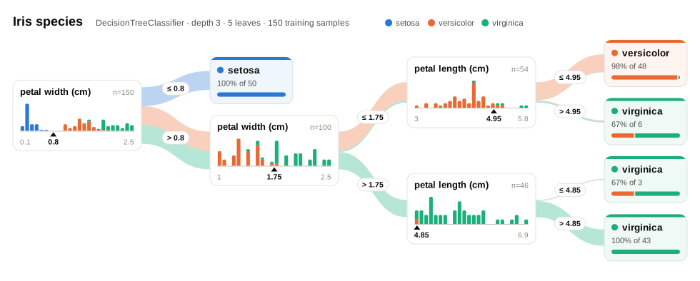
01
DecisionTreeClassifierlive
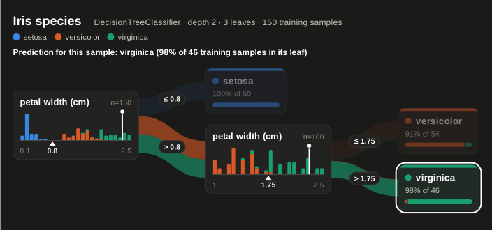
d = datasets.load_iris(as_frame=True)
X, y = d.data, d.target
clf = DecisionTreeClassifier(max_depth=3, random_state=0).fit(X, y)
fig = viz.draw(clf, X, y, class_names=d.target_names, title="Iris species")
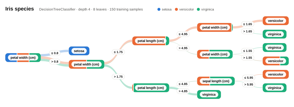
Simple mode
02
DecisionTreeClassifierlive
d = datasets.load_iris(as_frame=True)
X, y = d.data, d.target
clf = DecisionTreeClassifier(max_depth=4, random_state=0).fit(X, y)
fig = viz.draw(clf, X, y, class_names=d.target_names, simple=True, title="Iris species")
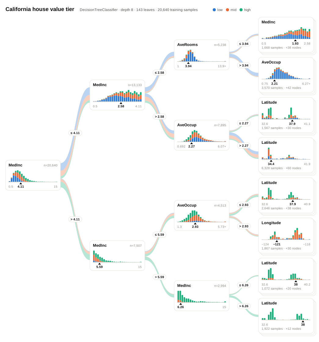
A bigger tree
03
DecisionTreeClassifierlive
d = datasets.fetch_california_housing(as_frame=True)
X = d.data
y = pd.qcut(d.target, 3, labels=False) # value tier: low / mid / high
clf = DecisionTreeClassifier(max_depth=8, min_samples_leaf=50, random_state=0).fit(X, y)
fig = viz.draw(clf, X, y, class_names=["low", "mid", "high"], max_depth=3,
title="California house value tier")
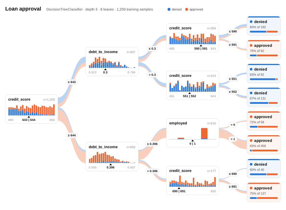
Binary and integer features
04
DecisionTreeClassifierlive
X, y = loan_data() # synthetic credit data, see docs/pages/viz_gallery.py
clf = DecisionTreeClassifier(max_depth=3, min_samples_leaf=20, random_state=0).fit(X, y)
fig = viz.draw(clf, X, y, class_names={0: "denied", 1: "approved"}, title="Loan approval")
Regression and one sample's decision path
05
DecisionTreeRegressorlive
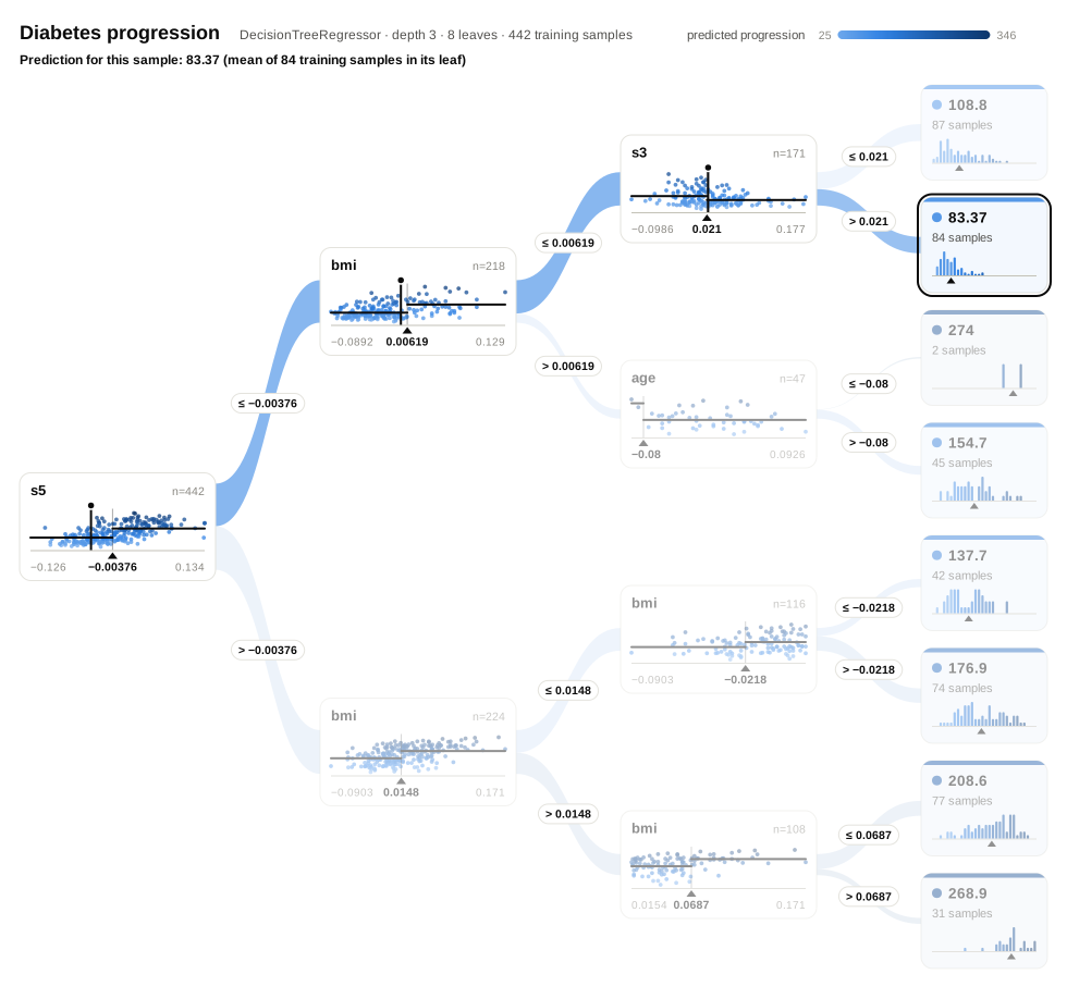
d = datasets.load_diabetes(as_frame=True)
X, y = d.data, d.target
reg = DecisionTreeRegressor(max_depth=3, random_state=0).fit(X, y)
fig = viz.draw(reg, X, y, x=X.iloc[7], target_name="progression", title="Diabetes progression")
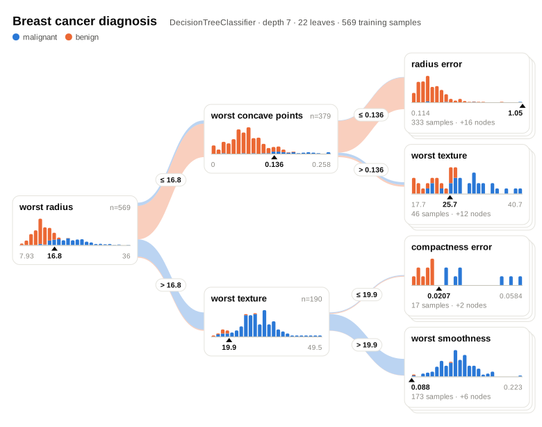
d = datasets.load_breast_cancer(as_frame=True)
X, y = d.data, d.target
clf = DecisionTreeClassifier(random_state=0).fit(X, y) # unrestricted depth
fig = viz.draw(clf, X, y, class_names=d.target_names, max_depth=2, title="Breast cancer diagnosis")
Many classes, compact style
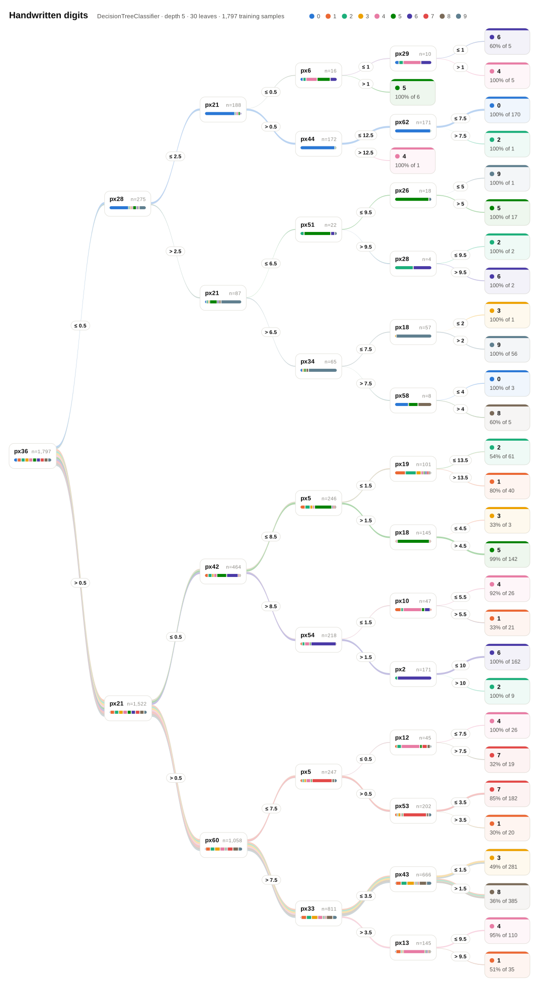
10
DecisionTreeClassifierlive
d = datasets.load_digits()
clf = DecisionTreeClassifier(max_depth=5, random_state=0).fit(d.data, d.target)
fig = viz.draw(clf, feature_names=[f"px{i}" for i in range(64)], title="Handwritten digits")
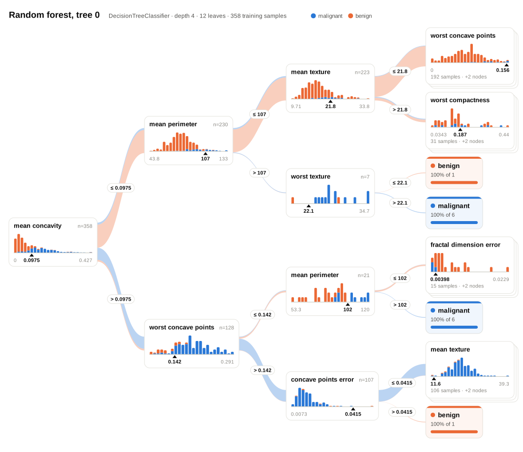
One tree from a random forest
11
RandomForestClassifier
d = datasets.load_breast_cancer(as_frame=True)
X, y = d.data, d.target
rf = RandomForestClassifier(n_estimators=50, max_depth=4, random_state=0).fit(X, y)
fig = viz.draw(rf.estimators_[0], X, y, feature_names=list(X.columns),
class_names=d.target_names, max_depth=3, title="Random forest, tree 0")
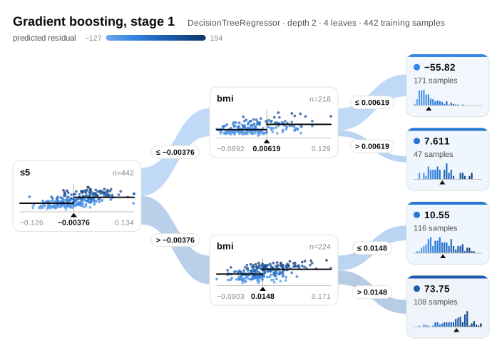
A gradient boosting stage
12
GradientBoostingRegressor
d = datasets.load_diabetes(as_frame=True)
X, y = d.data, d.target
gbm = GradientBoostingRegressor(n_estimators=20, max_depth=2, random_state=0).fit(X, y)
resid = y - y.mean() # what the first stage is fit to
fig = viz.draw(gbm.estimators_[0, 0], X, resid, feature_names=list(X.columns),
target_name="residual", title="Gradient boosting, stage 1")
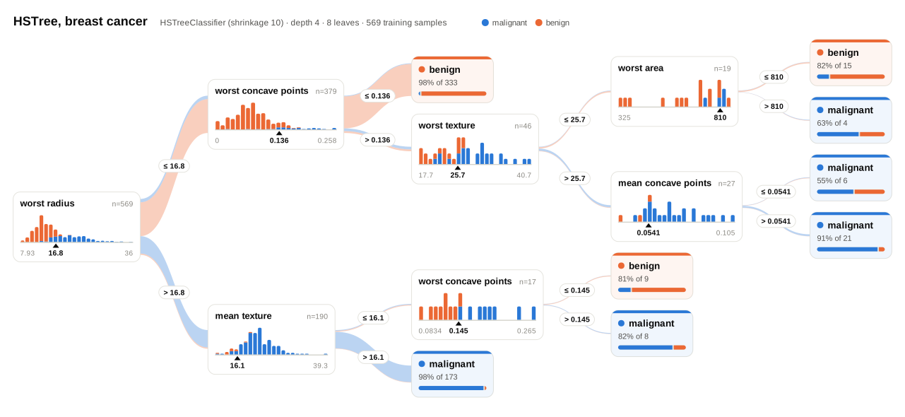
Hierarchical shrinkage (HSTree)
13
HSTreeClassifierlive
X, y = cancer.data, cancer.target
model = imodels.HSTreeClassifier(max_leaf_nodes=8, reg_param=10).fit(X, y)
kw = dict(class_names=["malignant", "benign"], title="HSTree, breast cancer")
fig = viz.draw(model, X, y, **kw)
page = viz.interactive(model, X, y, **kw)
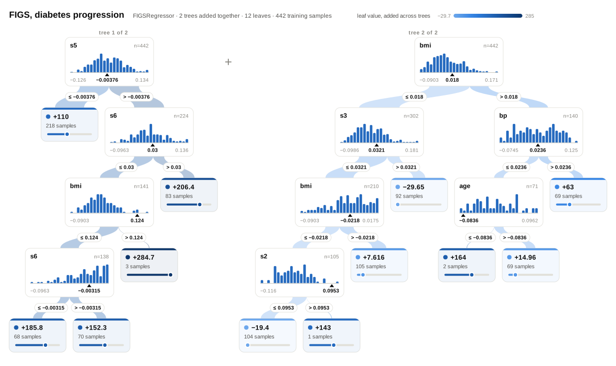
FIGS: a sum of trees
14
FIGSRegressorlive
X, y = diabetes.data, diabetes.target
model = imodels.FIGSRegressor(max_rules=10).fit(X, y)
kw = dict(title="FIGS, diabetes progression")
fig = viz.draw(model, X, y, **kw)
page = viz.interactive(model, X, y, **kw)
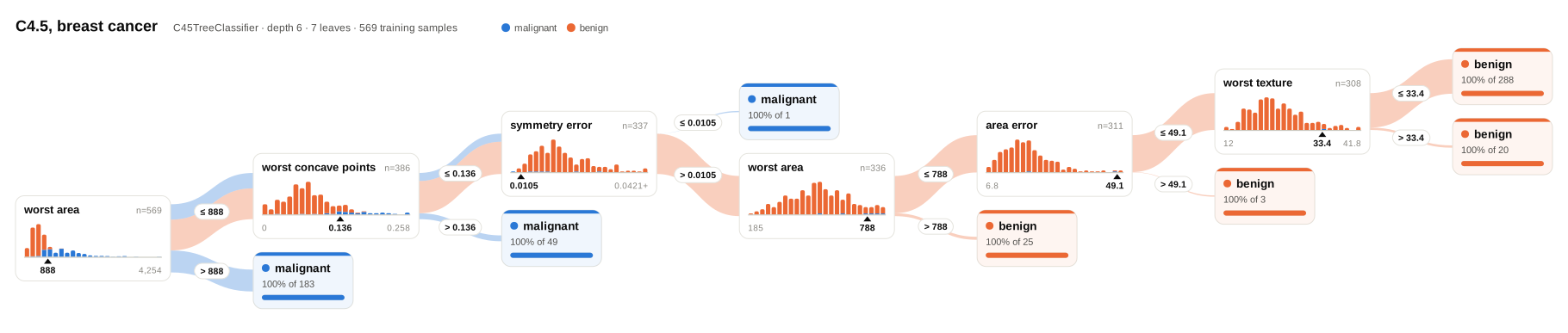
C4.5 tree
15
C45TreeClassifierlive
X, y = cancer.data, cancer.target
model = imodels.C45TreeClassifier(max_rules=6).fit(X, y)
kw = dict(class_names=["malignant", "benign"], title="C4.5, breast cancer")
fig = viz.draw(model, X, y, **kw)
page = viz.interactive(model, X, y, **kw)
Iterative random forest (IRF)
16
IRFClassifierlive
X, y = cancer.data, cancer.target
model = imodels.IRFClassifier(n_estimators=20, max_depth=3, random_state=0).fit(X, y)
kw = dict(class_names=["malignant", "benign"], title="IRF, breast cancer", max_trees=3)
fig = viz.draw(model, X, y, **kw)
page = viz.interactive(model, X, y, **kw)
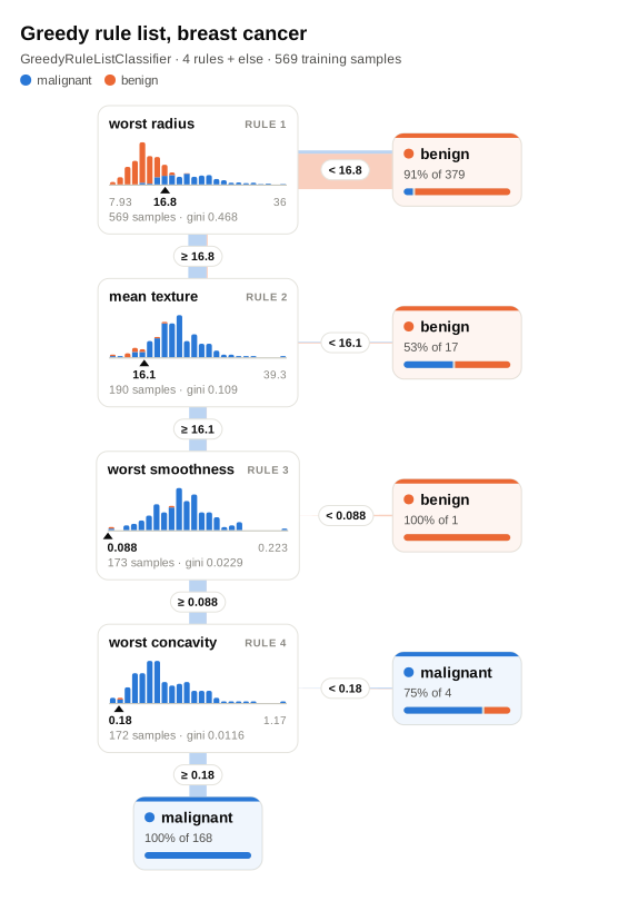
Greedy rule list
17
GreedyRuleListClassifierlive
X, y = cancer.data, cancer.target
model = imodels.GreedyRuleListClassifier(max_depth=4).fit(X, y)
kw = dict(class_names=["malignant", "benign"], title="Greedy rule list, breast cancer")
fig = viz.draw(model, X, y, **kw)
page = viz.interactive(model, X, y, **kw)
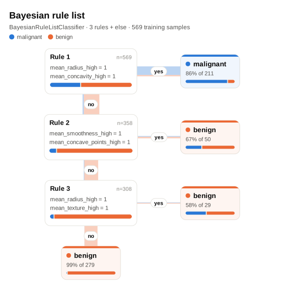
Bayesian rule list
18
BayesianRuleListClassifierlive
X = (cancer.data.iloc[:, :8] > cancer.data.iloc[:, :8].median()).astype(int)
X.columns = [c.replace(" ", "_") + "_high" for c in X.columns]
y = cancer.target
model = imodels.BayesianRuleListClassifier(max_iter=2000, n_chains=2, random_state=0).fit(X, y)
kw = dict(class_names=["malignant", "benign"], title="Bayesian rule list")
fig = viz.draw(model, X, y, **kw)
page = viz.interactive(model, X, y, **kw)
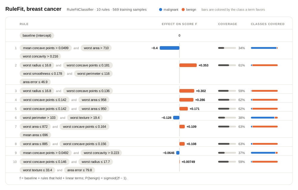
RuleFit
19
RuleFitClassifierlive
X, y = cancer.data, cancer.target
model = imodels.RuleFitClassifier(max_rules=12, random_state=0).fit(X, y)
kw = dict(class_names=["malignant", "benign"], title="RuleFit, breast cancer")
fig = viz.draw(model, X, y, **kw)
page = viz.interactive(model, X, y, **kw)
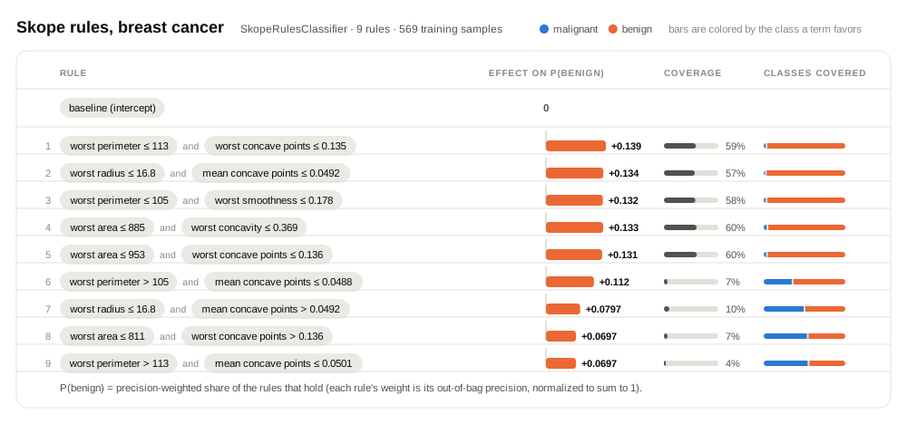
Skope rules
20
SkopeRulesClassifierlive
X, y = cancer.data, cancer.target
model = imodels.SkopeRulesClassifier(n_estimators=5, max_depth=2, random_state=0).fit(X, y)
kw = dict(class_names=["malignant", "benign"], title="Skope rules, breast cancer")
fig = viz.draw(model, X, y, **kw)
page = viz.interactive(model, X, y, **kw)
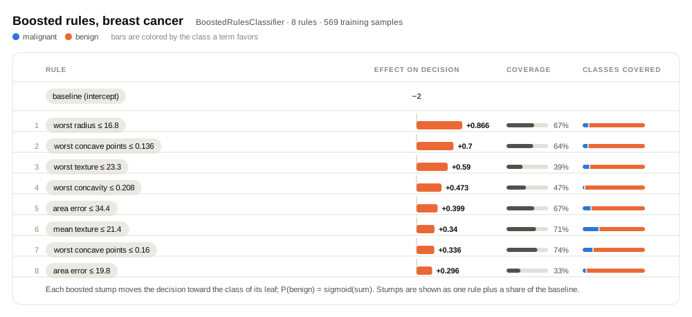
Boosted rules
21
BoostedRulesClassifierlive
X, y = cancer.data, cancer.target
model = imodels.BoostedRulesClassifier(n_estimators=8, random_state=0).fit(X, y)
kw = dict(class_names=["malignant", "benign"], title="Boosted rules, breast cancer")
fig = viz.draw(model, X, y, **kw)
page = viz.interactive(model, X, y, **kw)
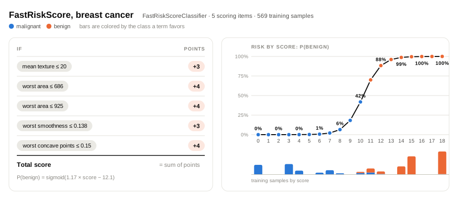
FastRiskScore
22
FastRiskScoreClassifierlive
X, y = cancer.data, cancer.target
model = imodels.FastRiskScoreClassifier(k=5, time_limit=20).fit(X, y)
kw = dict(class_names=["malignant", "benign"], title="FastRiskScore, breast cancer")
fig = viz.draw(model, X, y, **kw)
page = viz.interactive(model, X, y, **kw)
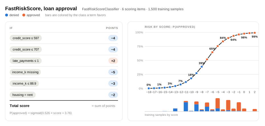
FastRiskScore with categories and missing values
23
FastRiskScoreClassifierlive
X, y = loans_with_categories() # credit data with a 'housing' column and missing incomes
model = imodels.FastRiskScoreClassifier(k=6, time_limit=30).fit(X, y)
kw = dict(class_names=["denied", "approved"], title="FastRiskScore, loan approval")
fig = viz.draw(model, X, y, **kw)
page = viz.interactive(model, X, y, **kw)
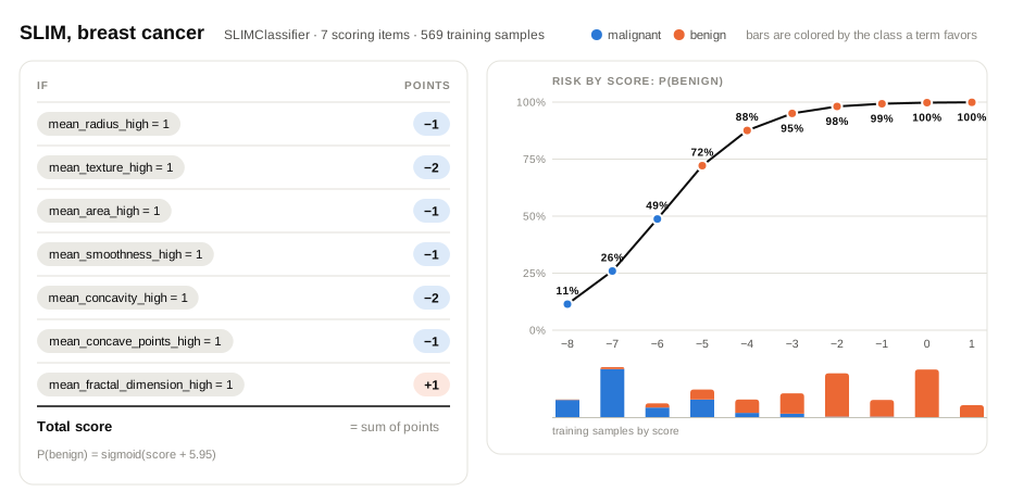
SLIM
24
SLIMClassifierlive
X = (cancer.data.iloc[:, :10] > cancer.data.iloc[:, :10].median()).astype(int)
X.columns = [c.replace(" ", "_") + "_high" for c in X.columns]
y = cancer.target
model = imodels.SLIMClassifier(alpha=0.5).fit(X, y)
kw = dict(class_names=["malignant", "benign"], title="SLIM, breast cancer")
fig = viz.draw(model, X, y, **kw)
page = viz.interactive(model, X, y, **kw)
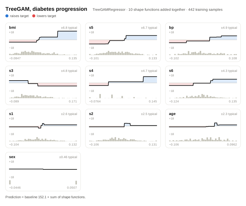
TreeGAM
25
TreeGAMRegressorlive
X, y = diabetes.data, diabetes.target
model = imodels.TreeGAMRegressor(n_boosting_rounds=20).fit(X, y)
kw = dict(title="TreeGAM, diabetes progression")
fig = viz.draw(model, X, y, **kw)
page = viz.interactive(model, X, y, **kw)
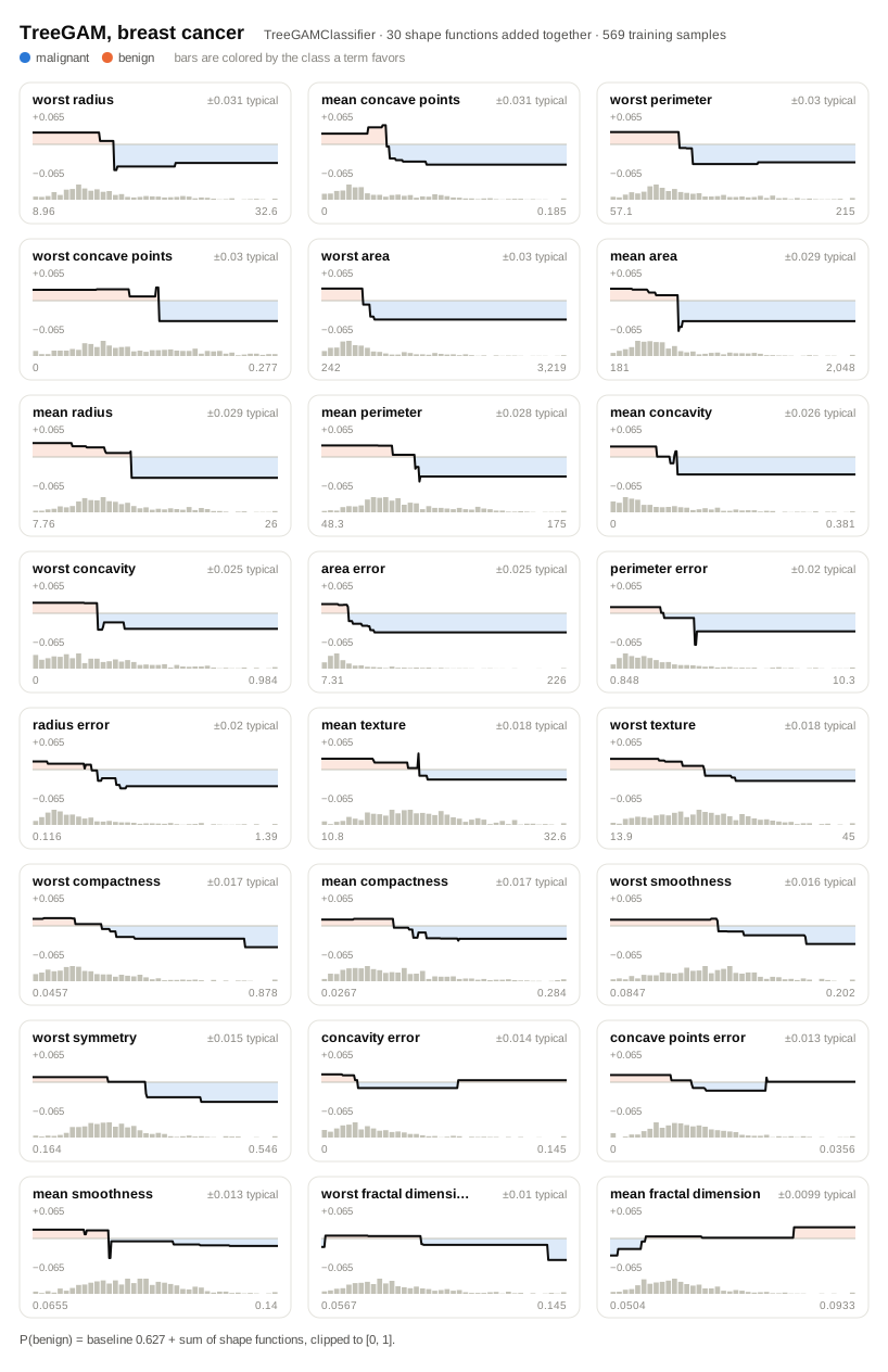
TreeGAM classifier
26
TreeGAMClassifierlive
X, y = cancer.data, cancer.target
model = imodels.TreeGAMClassifier(n_boosting_rounds=20).fit(X, y)
kw = dict(class_names=["malignant", "benign"], title="TreeGAM, breast cancer")
fig = viz.draw(model, X, y, **kw)
page = viz.interactive(model, X, y, **kw)
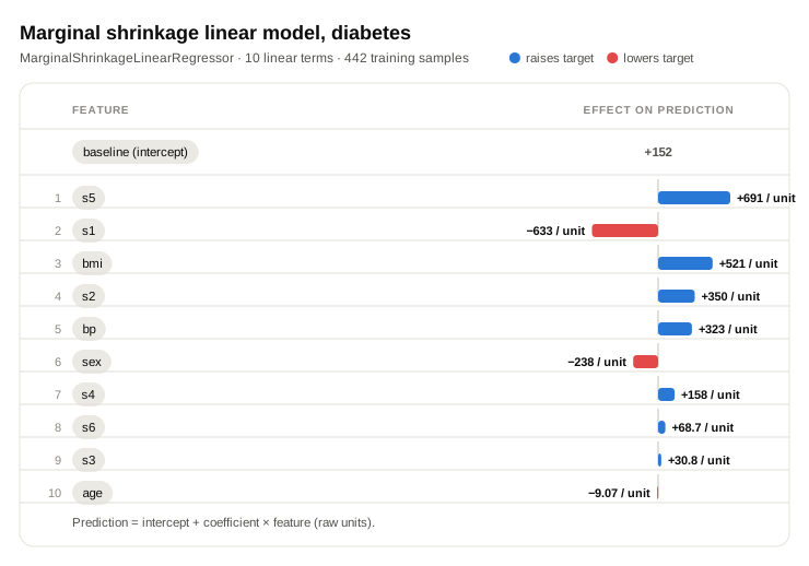
Linear model with marginal shrinkage
27
MarginalShrinkageLinearModelRegressorlive
X, y = diabetes.data, diabetes.target
model = imodels.MarginalShrinkageLinearModelRegressor().fit(X, y)
kw = dict(title="Marginal shrinkage linear model, diabetes")
fig = viz.draw(model, X, y, **kw)
page = viz.interactive(model, X, y, **kw)
Random forest
28
RandomForestClassifierlive
from sklearn.ensemble import RandomForestClassifier
X, y = cancer.data, cancer.target
model = RandomForestClassifier(n_estimators=50, max_depth=3, random_state=0).fit(X, y)
kw = dict(class_names=["malignant", "benign"], title="Random forest, breast cancer", max_trees=3)
fig = viz.draw(model, X, y, **kw)
page = viz.interactive(model, X, y, **kw)
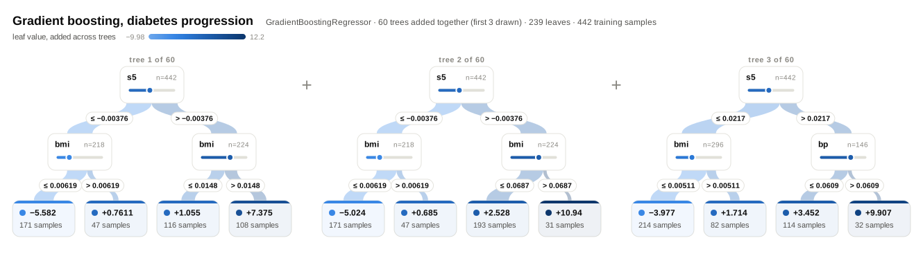
Gradient boosting
29
GradientBoostingRegressorlive
X, y = diabetes.data, diabetes.target
model = GradientBoostingRegressor(n_estimators=60, max_depth=2, random_state=0).fit(X, y)
kw = dict(title="Gradient boosting, diabetes progression", max_trees=3)
fig = viz.draw(model, X, y, **kw)
page = viz.interactive(model, X, y, **kw)
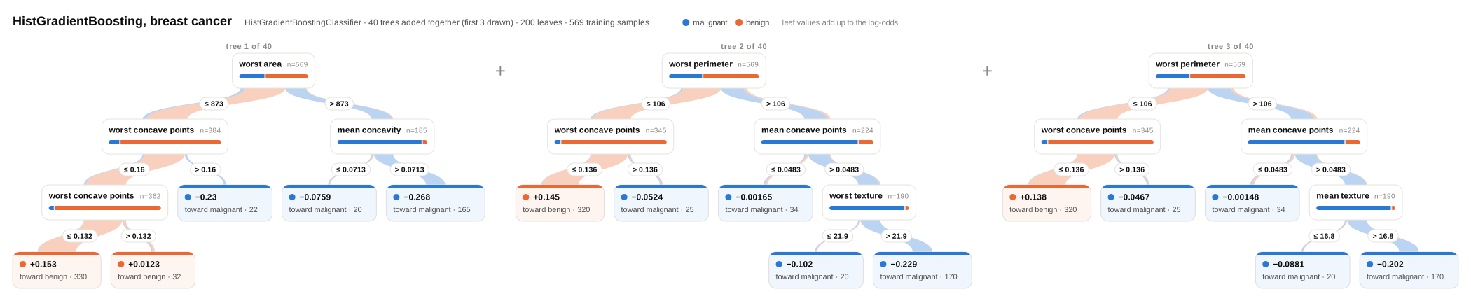
Histogram gradient boosting
30
HistGradientBoostingClassifierlive
from sklearn.ensemble import HistGradientBoostingClassifier
X, y = cancer.data, cancer.target
model = HistGradientBoostingClassifier(max_iter=40, max_leaf_nodes=5, random_state=0).fit(X, y)
kw = dict(class_names=["malignant", "benign"], title="HistGradientBoosting, breast cancer", max_trees=3)
fig = viz.draw(model, X, y, **kw)
page = viz.interactive(model, X, y, **kw)
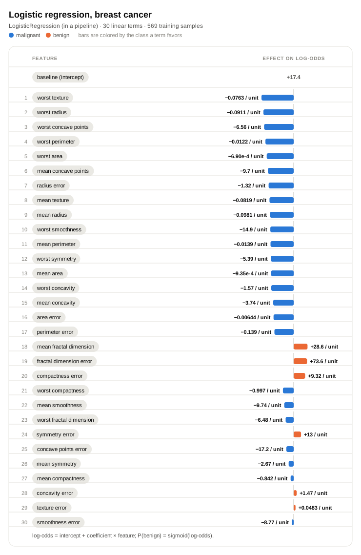
Logistic regression in a pipeline
31
LogisticRegressionlive
from sklearn.linear_model import LogisticRegression
from sklearn.pipeline import make_pipeline
from sklearn.preprocessing import StandardScaler
X, y = cancer.data, cancer.target
model = make_pipeline(StandardScaler(), LogisticRegression(C=0.05, max_iter=2000)).fit(X, y)
kw = dict(class_names=["malignant", "benign"], title="Logistic regression, breast cancer")
fig = viz.draw(model, X, y, **kw)
page = viz.interactive(model, X, y, **kw)
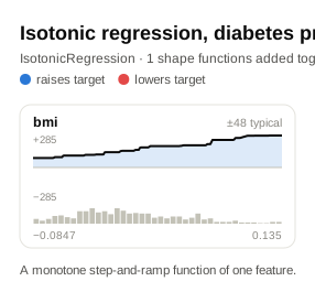
Isotonic regression
32
IsotonicRegressionlive
from sklearn.isotonic import IsotonicRegression
X, y = diabetes.data[["bmi"]], diabetes.target
model = IsotonicRegression(out_of_bounds="clip").fit(X["bmi"], y)
kw = dict(title="Isotonic regression, diabetes progression by bmi")
fig = viz.draw(model, X, y, **kw)
page = viz.interactive(model, X, y, **kw)
Generated by
docs/pages/viz_gallery.py on 2026-10-06.