6.7. logic#
6.7.1. logical agents - 7.1-7.7 (omitting 7.5.2)#
knowledge-based agents - intelligence is based on reasoning that operates on internal representations of knowledge
deductive - general-to-specific
inductive - specific-to-general
3 steps: given a percept, the agent
adds the percept to its knowledge base (KB)
asks the knowledge base for the best action
tells the knowledge base that it has taken that action
2 approaches
declarative approach - tell sentences until agent knows how to operate
know something, can verbalize it
procedural approach - encodes desired behaviors as program code
intuitively know how to do it (ex. riding a bike)
ex. Wumpus World
logical entailment between sentences
\(A \vDash B\) means B follows logically from A (A implies B)
logical inference - showing entailment
model checking - try everything to see if A \(\implies\) B
this is sound = truth-preserving
complete - can derive any sentence that is entailed
TT-ENTAILS
recursively enumerate all sentences by assigning true, false to each variable
check if these are valid within the KB
if they are, they must also match the query (otherwise return false)
grounding - connection between logic and real environment (usually sensors)
theorem properties
validity - tautalogy - true under all models
satisfiable - true under some model
ex. boolean-SAT
monotonicity - set of implications can only increase as info is added to the knowledge base
if \(KB \implies A\) then \(KB \land B \implies A\)
6.7.1.1. theorem proving#
resolution rule - resolves different rules with each other - leads to complete inference procedure
CNF - conjunctive normal form - conjunction (and) of clauses (with ors)
ex: \( ( \neg A \lor B) \land \neg C \land (D \lor E)\)
anything can be expressed as this
horn clause - at most one positive
definite clause - disjunction of literals with exactly one positive: ex. (\(A \lor \neg B \lor \neg C\))
goal clause - no positive: ex. (\(\neg A \lor \neg B \lor \neg C\))
benefits
easy to understand
forward-chaining / backward-chaining are applicable
deciding entailment is linear in size (KB)
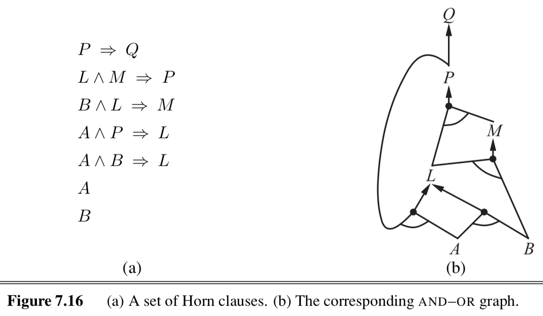
forward/backward chaining: checks if q is entailed by KB of definite clauses
data-driven
keep adding until query is added or nothing else can be added

backward chaining works backwards from the query
goal-driven
keep going until get back to known facts
checking satisfiability
complete backtracking
davis-putnam algorithm = DPLL - like TT-entails with 3 improvements
early termination
pure symbol heuristic - pure symbol appears with same sign in all clauses, can just set it to the proper value
unit clause heuristic - clause with just one literal or one literal not already assigned false
other improvements (similar to search)
component analysis
variable and value ordering
intelligent backtracking
random restarts
clever indexing
local search
evaluation function can just count number of unsatisfied clauses (MIN-CONFLICTS algorithm for CSPs)
WALKSAT - randomly chooses between flipping based on MIN-CONFLICTS and randomly
runs forever if no soln
underconstrained problems are easy to find solns
satisfiability threshold conjecture - for random clauses, probability of satisfiability goes to 0 or 1 based on ratio of clauses to symbols
hardest problems are at the threshold
6.7.1.2. agents based on propositional logic#
fluents = state variables that change over time
can index these by time
effect axioms - specify the effect of an action at the next time step
frame axioms - assert that all propositions remain the same under actions
succesor-state axiom: \(F^{t+1} \iff ActionCausesF^t \lor (F^t \land -ActionCausesNotF^t )\)
ex. \(HaveArrow^{t+1} \iff (HaveArrow^t \land \neg Shoot^t)\)
makes things stay the same unles something changes
state-estimation: keep track of belief state
can just use 1-CNF (conjunctions of literals: ex. \(WumpusAlive \land L_2 \land B\))
1-CNF includes all states that are in fact possible given the full percept history
conservative approximation - contains belief state, but also extraneous stuff
planning
could use \(A^*\) with entailment
otherwise, could use SATPLAN
SATPLAN - how to make plans for future actions that solve the goal by propositional inference
basic idea
make assertions
transitions up to some max time \(t_{final}\)
assert that goal is achieved at time \(t_{final}\) (ex. havegold)
present this to a SAT solver
must add precondition axioms - states that action occurrence requires preconditions to be satisfied
ex. can’t shoow without arrow
must add action exclusion axioms - one action at a time
ex. can’t shoot and move at once
6.7.2. first-order logic - 8.1-8.3.3#

basically added objects, relations, quantifiers (\(\exists, \forall\))
declarative language - semantics based on a truth relation between sentences and possible worlds
has compositionality - meaning decomposes
sapir-whorf hypothesis - understanding of the world is influenced by the language we speak
3 elements
objects - john (cannot appear by itself, need boolean value)
relations - set of tuples (ex. brother(richard, john))
functions - only one value for given input (ex. leftLeg(john))
sentences return true or false
combine these things
first-order logic assumes more about the world than propositional logic
epistemological commitments - the possible states of knowledge that a logic allows with respect to each fact
higher-order logic - views relations and functions as objects in themselves
first-order consists of symbols
constant symbols - stand for objects
predicate symbols - stand for relations
function symbols - stand for functions
arity - fixes number of args
term - logical expresision tha refers to an object
atomic sentence - formed from a predicate symbol optionally followed by a parenthesized list of terms
true if relation holds among objects referred to by the args
ex. Brother(Richard, John)
interpretation - specifies exactly which objects, relations and functions are referred to by the symbols
6.7.3. inference in first-order logic - 9.1-9.4#
propositionalization - can convert first-order logic to propositional logic and do propositional inference
universal instantiation - we can infer any sentence obtained by substituting a ground term for the variable
replace “forall x” with a specific x
existential instantiation - variable is replaced by a new constant symbol
replace “there exists x” with a specific x that give a name (called the Skolem constant)
only need finite subset of propositionalized KB - can stop nested functions at some depth
semidecidable - algorithms exist that say yes to every entailed sentence, but no algorithm exists that also says no to every nonentailed sentence
generalized modus ponens
unification - finding substitutions that make different logical expressions look identical
UNIFY(Knows(John,x), Knows(x,Elizabeth)) = fail .
use different x’s - standardizing apart
want most general unifier
need occur check - S(x) can’t unify with S(S(x))
storage and retrieval
STORE(s) - stores a sentence s into the KB
FETCH(q) - returns all unifiers such that the query q unifies with some sentence in the KB
only try to unify reasonable facts using indexing
query such as Employs(IBM, Richard)
all possible unifying queries form subsumption lattice
forward chaining: start w/ atomic sentences + apply modus ponens until no new inferences can be made
first-order definite clauses - (remember this is a type of Horn clause)
Datalog - language restricted to first-order definite clauses with no function symbols
simple forward-chaining: FOL-FC-ASK - may not terminate if not entailed
pattern matching is expensive
rechecks every rule
generates irrelevant facts
efficient forward chaining (solns to above problems)
conjuct odering problem - find an ordering to solve the conjuncts of the rule premise so the total cost is minimized
requires heuristics (ex. minimum-remaining-values)
incremental forward chaining - ignore redundant rules
every new fact inferred on iteration t must be derived from at least one new fact inferred on iteration t-1
rete algorithm was first to do this
irrelevant facts can be ignored by backward chaining
could also use deductive database to keep track of relevant variables
backward-chaining
simple backward-chaining: FOL-BC-ASK
is a generator - returns multiple times, each giving one possible result
like DFS - might go forever
logic programming: algorithm = logic + control
ex. prolog
a lot more here
can have parallelism
redudant inference / infinite loops because of repeated states and infinite paths
can use memoization (similar to the dynamic programming that forward-chaining does)
generally easier than converting it into FOLD
constraint logic programming - allows variables to be constrained rather than bound
allows for things with infinite solns
can use metarules to determine which conjuncts are tried first
6.7.4. classical planning 10.1-10.2#
planning - devising a plan of action to achieve one’s goals
Planning Domain Definition Language (PDDL) - uses factored representation of world
closed-world assumption - fluents that aren’t present are false
solving the frame problem: only specify result of action in terms of what changes
requires 4 things (like search w/out path cost function)
initial state
actions
transitions
goals
no quantifiers
set of ground (variable-free) actions can be represented by a single action schema
like a method with precond and effect
\(Action(Fly(p, from, to))\):
PRECOND: \(At(p, from) \land Plane(p) \land Airport(from) \land Airport(to)\)
EFFECT: \(\neg At(p, from) \land At(p, to)\)
can only use variables in the precondition
problems
PlanSAT - try to find plan that solves a planning problem
Bounded PlanSAT - ask whether there is a soln of length k or less
6.7.4.1. algorithms for planning as state-space search#
forward (progression) state-space search
very inefficient
generally forward search is preferred because it’s easier to come up with good heuristics
backward (regression) relevant-states search
PDLL makes it easy to regress from a state description to the predecessor state description
start with a set of things in the goal (and any other fluent can hae any value)
keep track of a set at all points
in going backward, the effects that were added need not have been true before, but preconditions must have held before
heuristics
ex. ignore preconditions
ex. ignore delete lists - remove all negative literals
ex. state abstractions - many-to-one mapping from states \(\to\) abstract states
ex. ignore some fluents
decomposition
requires subgoal independence
6.7.5. fuzzy logic (lofti zadeh)#
ex blog post
fuzzy sets - instead of binary membership, can have partial membership \(\in [0, 1]\)
intersection of sets - usually take min over memberships
union of sets - usually take max over memberships
6.7.6. foundations of rule learning (furnkranz et al. 2014)#
terminology - rule has a condition (conjunctive of binary features) + a conclusion = implication
rule has 2 parts
antecedent = body - consists of conditions = binary features e.g. \(X_1 > 0\), \(X_2=0\)
conclusion = consequent* = head
rule \(r\) has length L
\(P, N\) - total positives / negatives in the data
\(TP =\hat P, FP =\hat N\) - positives / negatives covered (predicted) by a rule
\(FN, TN\) - positives / negatives not covered by a rule
\(\frac{TP}{P}\) = true positive rate = sensitivity
\(\frac{TN}{N}\) = true negative rate = specificity
rules evaluated with a heuristic \(H(\hat P, \hat N)\)
6.7.6.1. categorization of tasks (ch 1)#
historically, a lot of this was developed in the data mining community and gave rise to packages such as WEKA, RAPID-I, KNIME, ORANGE
historical algos: AQ2 (michalski, 1969), PRISM (cendrowska, 1987), CN2 (Clar & nibett, 1989), FOIL (quinlan, 1990), RIPPER (cohen 1995), PROGOL (muggleton, 1995), ALEPH (srinivasan, 1999) - entire rule workbench in one prolog file, OPUS (webb, 1955), CBA (lui et al. 1998)
predictive rules
propositional learning (just propositional logic) v relational learning (first-order logic) = relational data mining = inductive logic programming
concept learning - binary classification task
complete rule set \(\mathcal R\) - covers all positive examples (recall = 1)
consistent - rule set \(\mathcal R\) - covers no negative examples (precision = 1)
descriptive data mining - usually unsupervised, just learn patterns
associative rule learning is unsupervised descriptive (e.g. APRIORI)
here, both the conditions + conclusions can have many features
subgroup discovery is descriptive, but has a supervised label, so is actually like supervised clustering - goal is to learn subgroups with a significantly different class distribution than the entire population
relational learning - when data doesn’t fit in a table but is associated (e.g. customers have many purchases each)
6.7.6.2. basics of learning rules (ch 2)#
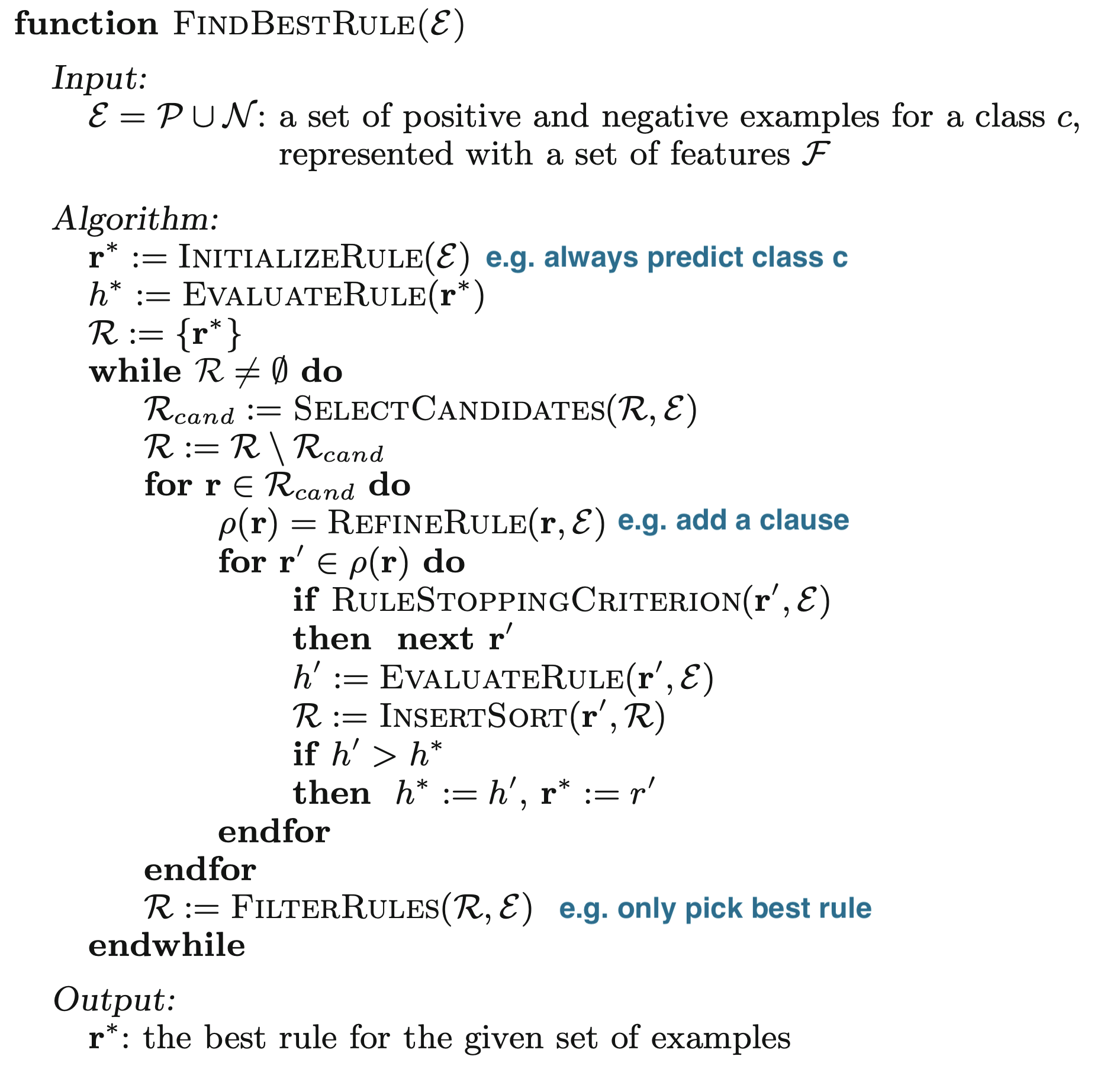
finding rules is basically a search problem
want to find best rules (generally bigger coverage, less complexity, higher accuracy)
can thing of it as searching on a refinement graph - each rule is a node and refinement operators connect rules
stopping criteria
threshold for some heuristic
making final prediction
final predictions can be made via majority vote, using most accurate rule, or averaging predictions.
algorithms
sequential covering (remove covered points after each rule)
6.7.6.3. (binary split) features (ch 4)#
here, feature means something binary that we split on
selector is smth of the form \(A_i \sim v_{i, j}\) where relation \(\sim\) is like \(=, >=, <=\)
can also be attribute sets (internal disjunctions) \(A_i \in \{v_1, v_2, v_3 \}\), intervals (range operators), or attribute sets (internal conjunctions)
can also be simple combinations of binary variables
relational features - function between features (e.g. length > height)
can have splits that are functions of previous splits (like a residual DNN connection)
many algorithms start by making a covering table = table of binary values for all possible (reasonable) splits for all features
split on all categorical features
split between all values of continuous features (or ordered discrete)
can compute relational features (e.g. \(A_1 - A_2\)) by just adding these as features
feature relevancy
\(pn-pair\): pair of training examples where one is positive and one is negative
totally irrelevant features - don’t distinguish between any positive/negative examples
a feature \(f_1\) is more relevant than another \(f_2\) if it separates all the \(pn\)-pairs that \(f_2\) does and more
can also manually set thresholds on TP, FP to decide irrelevance
missing values
different types
missing - was not measured but should have been
not applicable - e.g. pregnant for a male
don’t care - could be anything
basic strategies
delete incomplement examples
treat missing as special value
impute w/ mean/median/linear prediction
fill in prob distr. over missing val
pessimistic value strategy - imputed values shouldn’t differentiate between classes - set value so it doesn’t get used (e.g. false for positive class and true for neg class)
imprecise values - continuous values with noise
might want to test variables with \(\pm \delta\) handled with pessimistic value strategy
fuzzy rules - probabilistically split
6.7.6.4. relational features (ch 5)#
these kinds of task use relational background knowledge + databases
ex. from knowledge about things like female(X), parent(X, Y), learn that daughter(X, Y):= female(X) , parent(Y, X)
allow \(\forall, \exists\)
6.7.6.5. learning single rules (ch 6)#
search problem to maximize some criteria subject to some constraints
top-down - start with large cover then go to small
bottom-up - start with high-sensitivity, low cover rules then go larger

search algos
exhaustive search
hill-climbing = local-search - can make less myopic by considering multiple refinements at a time
beam-search - keep k best candidates
best-first search - beam search but keep all candidates
ordered search - prune the search space based on knowledge (e.g. order splitting values)
level-wise search (e.g. apriori) - generate in parallel all rules with a certain minimum quality
stochastic search - involves randomness
search directions: combine top-down (specialization) with bottom-up (generalization)
6.7.6.6. rule evaluation measures (ch 7)#
sometimes we only evaluate the quality of covered rules (e.g. rule list) whereas sometimes we evaluate quality of disjoint sets (e.g. both sides of decision tree split)
common heuristics are rules that cover a lots of samples or rules that are simple
equivalent heuristics: compatible heuristics \(H\), \(G\) rank rules in the same order (antagonistic rank rules in opposite order)
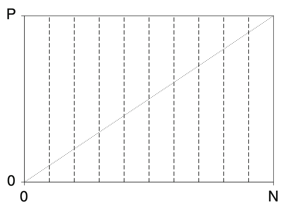
axes to evaluate rules (want to be close to top-left):

list of metrics (to maximize), all basically trade of recall / precision
\(Specificity = TN / N\)
\(Sensitivity = Recall = TP / P\)
\(Support = TP / (P + N)\)
\(CovDiff = TP - FP\)
equivalent to classification \(Accuracy=(TP + TN) / (P + N)\)
\(Coverage = (TP + FN) / (P + N)\) - fraction of points covered
\(RateDiff = TP / P - FP / N\)
this is equivalent to more general weighted relative accuracy \(LinCost = a \cdot TP - b \cdot FP\)
\(Precision = TP / \underbrace{(TP + FP)}_{\text{predicted pos}}\) (sometimes called confidence or rule accuracy)
RIPPER’s pruning heuristic \((TP - FP) / (TP + FP)\) is equivalent to precision
covering ratio \(TP / FP\) is equivalent to precision
information-theoretic measures
\(Info = -\log_2 Precision\)
\(Entropy = - (Prec \cdot \log_2 Prec + (1-Prec) \cdot \log_2 (1-Prec))\)
when \(TP \leq FN\), same as precision and when \(TP > FN\) opposite of precision
originally developed for case where we aren’t covering positive examples but rather predicting with majority class
also KL-divergence and Gini index
\(Laplace(r) = (TN + 1)/(TP+1+FP+1)\) - pad all the values by 1 to adjust scores when numbers are small
likelihood ratio statistic - compare distr in rule to distr in full dataset
complexity-based heuristics
\(Length\)
\(MDL(r) = I(r) + I(\epsilon|r)\)
hard to compute
