4.7. time series#
4.7.1. high-level#
4.7.1.1. basics#
usually assume points are equally spaced
modeling - for understanding underlying process or predicting
nice blog, nice tutorial, Time Series for scikit-learn People
noise, seasonality (regular / predictable fluctuations), trend, cycle
multiplicative models: time series = trend * seasonality * noise
additive model: time series = trend + seasonality + noise
stationarity - mean, variance, and autocorrelation structure do not change over time
endogenous variable = x = independent variable
exogenous variable = y = dependent variable
changepoint detection / Change detection - tries to identify times when the probability distribution of a stochastic process or time series changes
4.7.1.2. libraries#
skits library for forecasting
4.7.1.3. high-level modelling#
common methods
decomposition - identify each of these components given a time-series
ex. loess, exponential smoothing
frequency-based methods - e.g. look at spectral plot
(AR) autoregressive models - linear regression of current value of one or more prior values of the series
(MA) moving-average models - require fitting the noise terms
(ARMA) box-jenkins approach
moving averages
simple moving average - just average over a window
cumulative moving average - mean is calculated using previous mean
exponential moving average - exponentially weights up more recent points
prediction (forecasting) models
autoregressive integrated moving average (arima)
assumptions: stationary model
4.7.2. similarity measures#
An Empirical Evaluation of Similarity Measures for Time Series Classification (serra et al. 2014)
lock-step measures (Euclidean distance, or any norm)
can resample to make them same length
feature-based measures (Fourier coefficients)
euclidean distance over all coefs is same as over time-series, but we usually filter out high-freq coefs
can also use wavelets
model-based measures (auto-regressive)
compare coefs of an AR (or ARMA) model
elastic measures
dynamic time warping = DTW - optimally align in temporal domain to minimize accumulated cost
can also enforce some local window around points
Every index from the first sequence must be matched with one or more indices from the other sequence and vice versa
The first index from the first sequence must be matched with the first index from the other sequence (but it does not have to be its only match)
The last index from the first sequence must be matched with the last index from the other sequence (but it does not have to be its only match)
The mapping of the indices from the first sequence to indices from the other sequence must be monotonically increasing, and vice versa, i.e. if
j > iare indices from the first sequence, then there must not be two indicesl > kin the other sequence, such that indexiis matched with indexland indexjis matched with indexk, and vice versa
edit distance EDR
time-warped edit distance - TWED
minimum jump cost - MJC
4.7.3. book1 (A course in Time Series Analysis) + book2 (Intro to Time Series and Forecasting)#
4.7.3.1. ch 1#
when errors are dependent, very hard to distinguish noise from signal
usually in time-series analysis, we begin by de-trending the data and analyzing the residuals
ex. assume linear trend or quadratic trend and subtract that fit (or could include sin / cos for seasonal behavior)
ex. look at the differences instead of the points (nth order difference removes nth order polynomial trend). However, taking differences can introduce dependencies in the data
ex. remove trend using sliding window (maybe with exponential weighting)
periodogram - in FFT, this looks at the magnitude of the coefficients (but loses the phase information)
4.7.3.2. ch 2 - stationary time series#
in time series, we never get iid data
instead we make assumptions
ex. the process has a constant mean (a type of stationarity)
ex. the dependencies in the time-series are short-term
autocorrelation plots: plot correlation of series vs series offset by different lags
formal definitions of stationarity for time series \(\{X_t\}\)
strict stationarity - the distribution is the same across time
second-order / weak stationarity - mean is constant for all t and, for any t and k, the covariance between \(X_t\) and \(X_{t+k}\) only depends on the lag difference k
In other words, there exists a function \(c: \mathbb Z \to \mathbb R\) such that for all t and k we have \(c(k) = \text{cov} (X_t, X_{t+k})\)
strict stationary and \(E|X_T^2| < \infty \implies\) second-order stationary
ergodic - stronger condition, says samples approach the expectation of functions on the time series: for any function \(g\) and shift \(\tau_1, ... \tau_k\):
\(\frac 1 n \sum_t g(X_t, ... X_{t+\tau_k}) \to \mathbb E [g(X_0, ..., X_{t+\tau_k} )]\)
causal - can predict given only past values (for Gaussian processes no difference)
4.7.3.3. ch 3 - linear time series#
note: can just assume all have 0 mean (otherwise add a constant)
AR model \(AR(p)\): $\( X_t = \sum_{i=1}^p \phi_i X_{t-i}+ \varepsilon_t \)$
\(\phi_1, \ldots, \phi_p\) are parameters
\(\varepsilon_t\) is white noise
stationary assumption places constraints on param values (e.g. processes in the \(AR(1)\) model with \(|\phi_1| \ge 1\) are not stationary)
looks just like linear regression, but is more complex
if we don’t account for issues, things can go wrong
model will not be stationary
model may be misspecified
\(E(\epsilon_t|X_{t-p}) \neq 0\)
this represents a set of difference equations, and as such, must have a solution
ex. \(AR(1)\) model - if \(|\phi| < 0\), then soln is in terms of past values of {\(\epsilon_t\)}, otherwise it is in terms of future values
ex. simulating - if we know \(\phi\) and \(\{\epsilon_t\}\), we still need to use the backshift operator to solve for \(\{ X_t \}\)
ex. \(AR(p)\) model - if \(\sum_j |\phi_j|\)< 1, and \(\mathbb E |\epsilon_t| < \infty\), then will have a causal stationary solution
backshift operator \(B^kX_t=X_{t-k}\)
solving requires using the backshift operator, because we need to solve for what all the residuals are
characteristic polynomial \(\phi(a) = 1 - \sum_{j=1}^p \phi_j a^j\)
\(\phi(B) X_t = \epsilon_t\)
\(X_t=\phi(B)^{-1} \epsilon_t\)
can represent \(AR(p)\) as a vector \(AR(1)\) using the vector \(\bar X_t = (X_t, ..., X_{t-p+1})\)
note: can reparametrize in terms of frequencies
MA model \(MA(q)\): \( X_t = \sum_{i=1}^q \theta_i \varepsilon_{t-i} + \varepsilon_t\)
\(\theta_1 ... \theta_q\) are params
\(\varepsilon_t\), \(\varepsilon_{t-1}\) are white noise error terms
harder to fit, because the lagged error terms are not visible (also means can’t make preds on new time-series)
\(E[\epsilon_t] = 0\), \(Var[\epsilon_t] = 1\)
much harder to estimate these parameters
\(X_t = \theta (B) \epsilon_t\) (assuming \(\theta_0=1\))
ARMA model: \(ARMA(p, q)\): \(X_t = \sum_{i=1}^p \phi_i X_{t-i} + \sum_{i=1}^q \theta_i \varepsilon_{t-i} + \varepsilon_t\)
\(\{X_t\}\) is stationary
\(\phi (B) X_t = \theta(B) \varepsilon_t\)
\(\phi(B) = 1 - \sum_{j=1}^p \phi_j B^j\)
\(\theta(B) = 1 + \sum_{j=1}^{q}\theta_jz^j\)
causal if \(\exists \{ \psi_j \}\) such that \(X_t = \sum_{j=0}^\infty \psi_j Z_{t-j}\) for all t
ARIMA model: \(ARIMA(p, d, q)\): - generalizes ARMA model to non-stationarity (using differencing)
4.7.3.4. ch 4 + 8 - the autocovariance function + parameter estimation#
estimation
pure autoregressive
Yule-walker
Burg estimation - minimizing sums of squares of forward and backward one-step prediction errors with respect to the coefficients
when \(q > 0\)
innovations algorithm
hannan-rissanen algorithm
autocovariance function: {\(\gamma(k): k \in \mathbb Z\)} where \(\gamma(k) = \text{Cov}(X_{t+h}. X_t) = \mathbb E (X_0 X_k)\) (assuming mean 0)
Yule-Walker equations (assuming AR(p) process): \(\mathbb E (X_t X_{t-k}) = \sum_{j=1}^p \phi_j \mathbb E (X_{t-j} X_{t-k}) + \underbrace{\mathbb E (\epsilon_tX_{t-k})}_{=0} = \sum_{j=1}^p \phi_j \mathbb E (X_{t-j} X_{t-k})\)
ex. MA covariance becomes 0 with lag > num params
can rewrite the Yule-Walker equations
\(\gamma(i) = \sum_{j=1}^p \phi_j \gamma(i -j)\)
\(\underline\gamma_p = \Gamma_p \underline \phi_p\)
\((\Gamma_p)_{i, j} = \gamma(i - j)\)
\(\hat{\Gamma}_p\) is nonegative definite (and nonsingular if there is at least one nonzero \(Y_i\))
\(\underline \gamma_p = [\gamma(1), ..., \gamma(p)]\)
\(\underline \phi_p = (\phi_1, ..., \phi_p)\)
this minimizes the mse \(\mathbb E [X_{t+1} - \sum_{j=1}^p \phi_j X_{t+1-j}]^2\)
use estimates to solve: \(\hat{\underline \phi}_p = \hat \Sigma_p^{-1} \hat{\underline r}_p \)
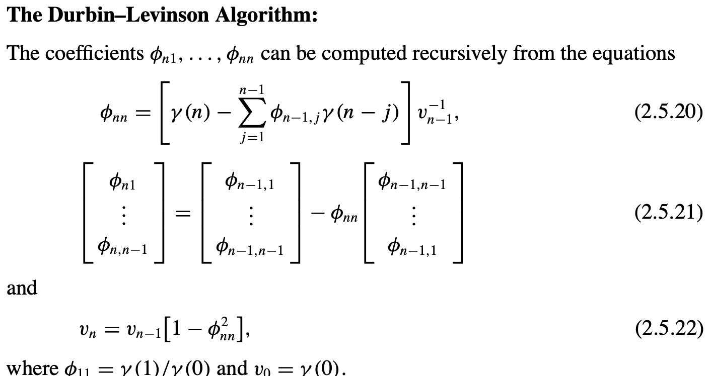
the innovations algorithm
set \(\hat X_1 = 0\)
innovations = one-step prediction errors \(U_n = X_n - \hat X _n\)
mle (ch 5.2)
eq. 5.2.9: Gaussian likelihood for an ARMA process
\(r_n = \mathbb E[(W_{n+1} - \hat W_{n+1})^2]\)
4.7.4. multivariate time-series ch 7#
vector-valued time-series has dependencies between variables across time
just modeling as univariate fails to take into account possible dependencies between the series
4.7.5. neural modeling#
see pytorch-forecasting for some new state-of-the-art models