3.8. chaos#

3.8.1. Normal forms of Hopf bifurcations#

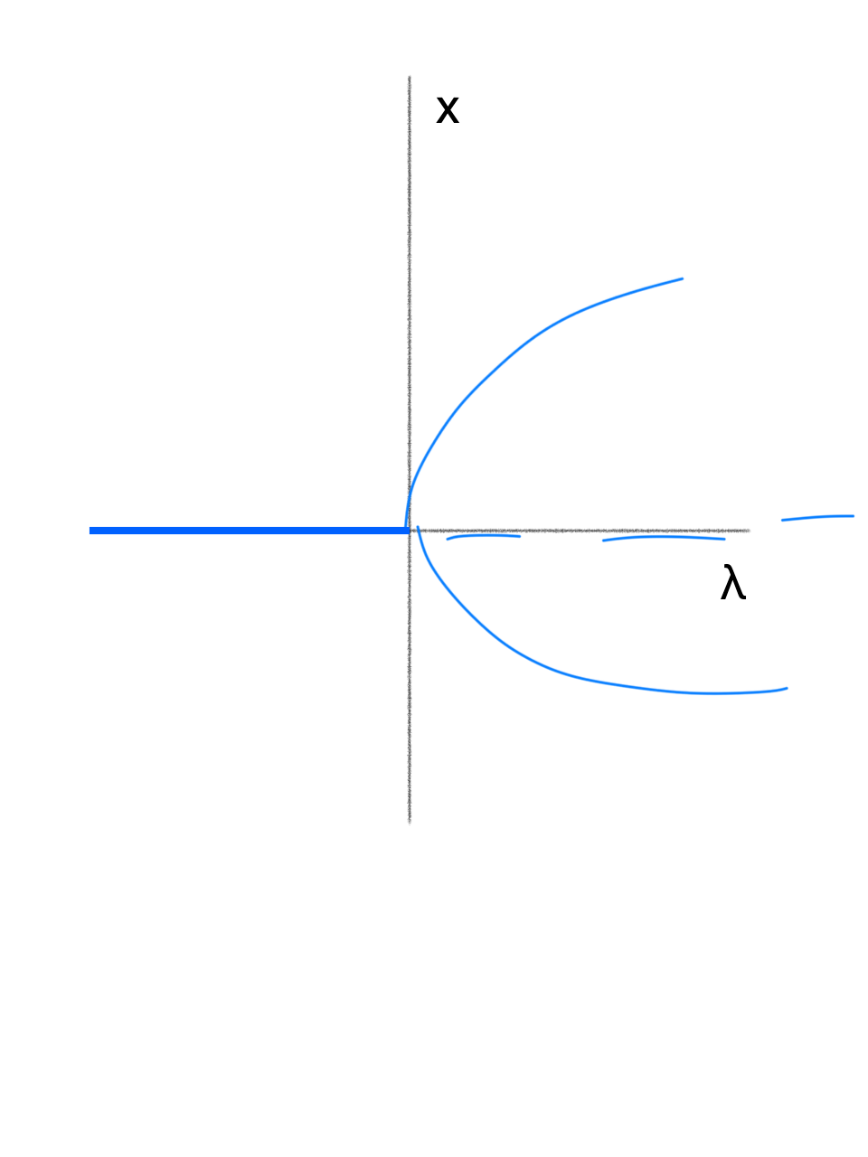
pitchfork: $$\dot{x} = \lambda x - x^3$$
subcritical pitchfork: $\dot{x} = \lambda x + x^3$
saddle node (turning point): $\dot{x} = \lambda - x^2$
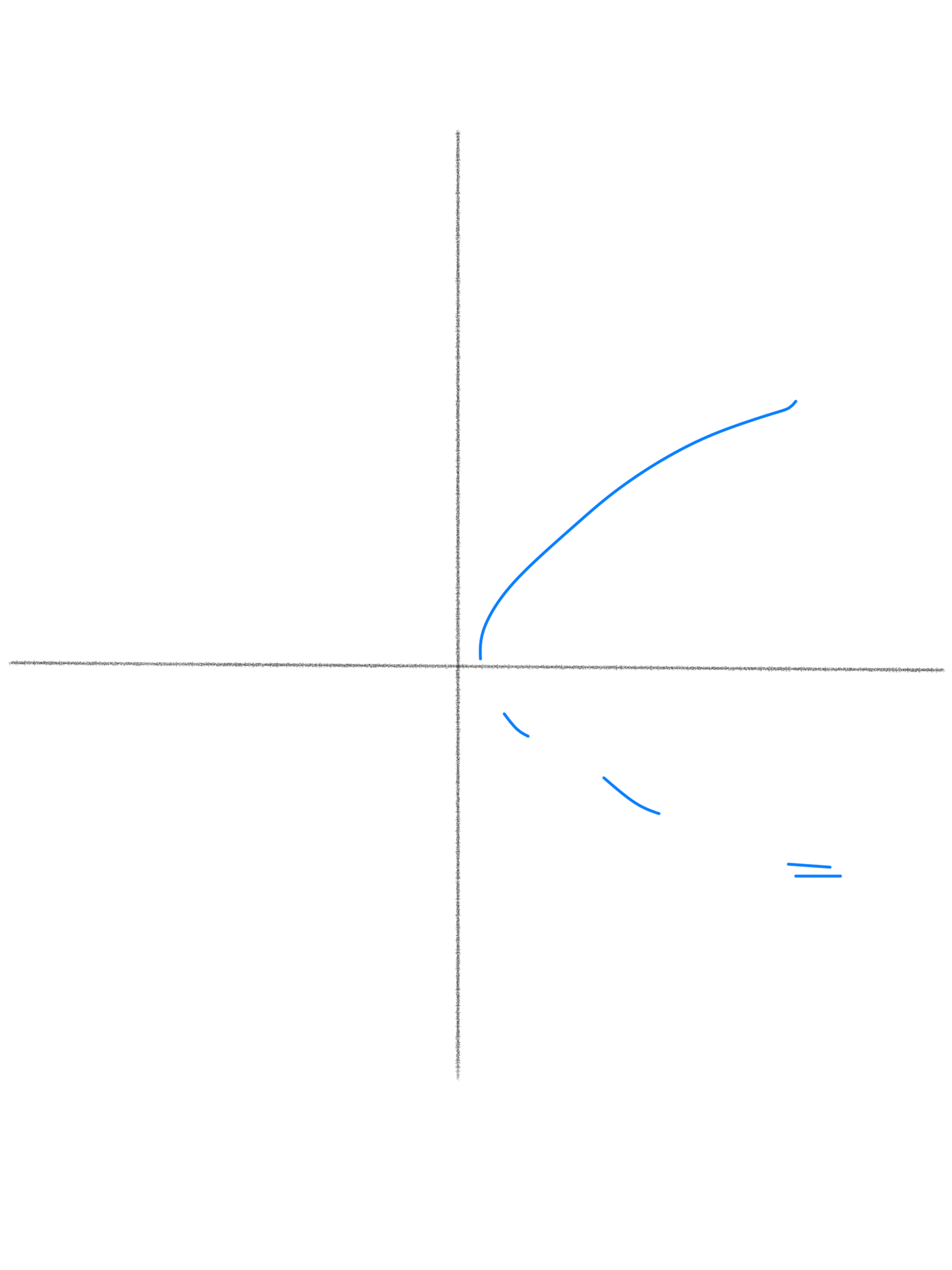
transcritical: $\dot{x} = \lambda x - x^2$

3.8.2. important figs#

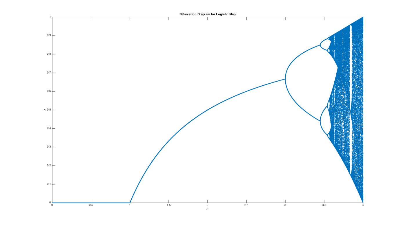
period-doubling (flip bifurcation) $f = \mu x (1-x) (f = \mu sin (\pi x) $ is similiar)
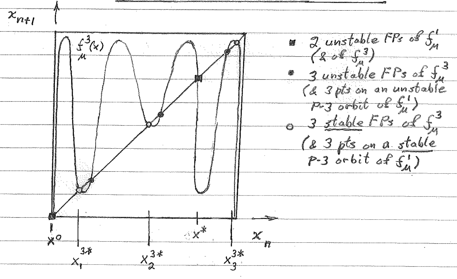
inverse tangent bifurcation - unstable and stable P-3 orbits coalesce, move slightly off bisector and becomes chaotic
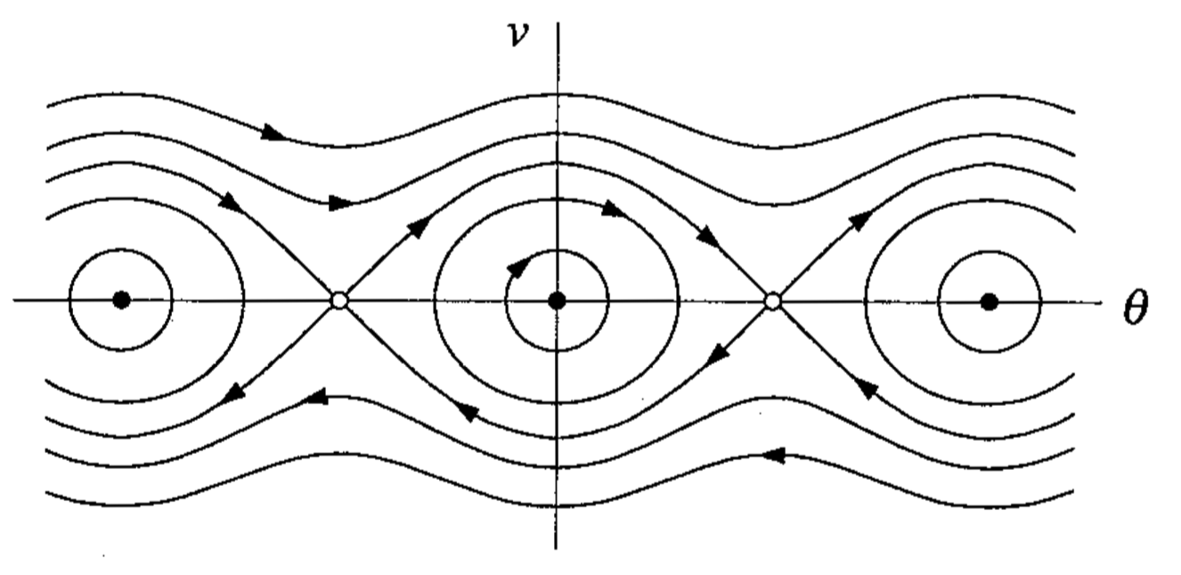
pendulum
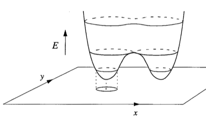
energy surface - trajectories run around the surface, not down it
Conservative systems: 6.5
- study Hamiltonian p. 187-188
Pendulum: 6.7
dynamics - study of things that evolve with time
chaos - deterministic, aperiodic, sensitive, long-term prediction impossible

phase space - has coordinates $x_1,...,x_n$
phase portrait - variable x-axis, derivative y-axis
bifurcation diagram - parameter x-axis, steady state y-axis
- draw separate graphs for these

first check - look for fixed points
for 1-D, if f’ $<$ 0 then stable
stable f.p. = all possible ICs in a.s.b.f.n. result in trajectories that remain in a.s.b.f.n. for all time
asymptotically stable f.p. - stable and approaches f.p. as $t\ra\infty$
hyperbolic f.p. - eigenvals aren’t strictly imaginary
bifurcation point of f.p. - point where num solutions change or phase portraits change significantly
globally stable - stable from any ICs
autonomous = f is a function of x, not t
we can always make a system autonomous by having $x_n$ = t, so $\dot{x_n}$ = 1
dimension = number of 1st order ODEs, dimension of phase-space
existence and uniqueness thm: if $\dot{x}$ and $\dot{x}'$ are continuous, then there is some unique solution
linearization - used to find stability of f.p.s
\[\begin{split} \dot{x} = f(x) &\\ \text{define }\delta x = (x-\bar{x}) \\ \dot{\delta x} = \frac{d}{dt}(x-\bar{x}) = \dot{x} = f(x) = f(\bar{x}+\delta x) \\ \dot{\delta x} =\cancelto{0}{f(\bar{x})} + \delta x f'(\bar{x}) + \cancelto{\text{0 by HGT iff f'!=0}}{O(x^2)} \\ \dot{\delta x} = \delta x f'(\bar{x}) \to \text{ now solve FOLDE} \\ \end{split}\]
solving Hopf: use polar to get $\dot{\rho}, \dot{\theta}$
multiply one thing by cos, one by sin, then add
$ \rho = \sqrt{x_1^2 + x_2^2} \\ \theta = tan^{-1}(\frac{x_2}{x_1})$
Hysterisis curve - S-shaped curve of fixed branches - ruler getting larger - snap bifurcation - both axes are parameters

3.8.3. Systems of Linear ODEs#

solutions are of the form $\underbar{x}(t) = \underbar{C}_1e^{\alpha_1 t} + \underbar{C}_2e^{\alpha_2 t}$
Eigenspaces: $E^S$ (stable), $E^U$ (unstable), $E^C$ (center - real part) - plot eigenvectors
how to solve these systems?
- solve eigenvectors
positive real part - goes out
negative real part - goes in
bifurcation requires 0 as eigenvalue
has imaginary component: spiral / focus
purely imaginary - center = stable, but not a.s.
finite velocity = $\frac{dRe(\alpha)}{d\lambda}$
change coordinates to polar
for $\lambda \geq 0$, solution is a stable L.C. (from either direction spirals into a circular orbit)
attracting - any trajectory that starts within $\delta$ of $\bar{\underbar{x}}$ evolves to $\bar{\underbar{x}}$ as t $\to \infty$ (it doesn’t have to remain within $\delta$ at all times
stable (Lyapanov stable) - any trajectory that starts within $\delta$ remains within $\varepsilon$ for all time ($\varepsilon$ is chosen first)
asymptotically stable - attracting and stable
hyperbolic f.p. - iff all eigenvals of the linearization of the nds about the f.p. have nonzero real parts \

3.8.4. Discrete Nonlinear Dynamical Systems#

functional iteration: $x_{n+m} = f^m(x_n)$ (apply f m times)
fixed point: $f(x^*)=x^*$
f.p. stable if $\|\frac{df}{dx}(x^*)\|<1$, unstable if $>$ 1
check n-orbit by checking nth derivative: $\frac{df^n}{dx}(x_i^*) = \prod_{i=1}^{n-1} \frac{df}{dx}(x_i^*)$
period-doubling bifurcations
self-stability - orbit for which the stability-determining derivative is zero. This means that the max of the map and the point at which the max occurs are in the orbit.
type I intermittency - exhibited by inverse tangent bifurcation
Feigenbaum sequence - period-doubling path to chaos, keep increasing parameter until period is chaotic

\begin{center} \begin{tabular}{ | m{4cm} | m{4cm} | } \hline \multicolumn{2}{|c|}{3D Attractors} \ \hline Type of Attractor & Sign of Exponents \ \hline Fixed Point & (-, -, -)\ Limit Cycle & (0, -, -) \ Torus & (0, 0, -) \ Strange Attractor & (+, 0, -) \ \hline \end{tabular} \end{center}

homoclinic orbit - connects unstable manifold of saddle point to its own stable manifold
- e.g. trajectory that starts and ends at the same fixed point
manifolds are denoted by a W (ex. $W^S$ is the stable manifold)
heteroclinic orbit - connects unstable manifold of fp to stable manifold of another fp \

3.8.5. Conservative Systems#

$F(x) = -\frac{dV}{dx}$ (by defn.)
$m\ddot{x}+\frac{dV}{dx}=0$, multiply by $\dot{x} \to \frac{d}{dt}[\frac{1}{2}m\dot{x}^2+V(x)]=0$
so total energy $E=\frac{1}{2}m\dot{x}^2+V(x)$
motion of pendulum: $\frac{d^2\theta}{dt^2}+\frac{g}{L}sin\theta=0$
nondimensionalize with $\omega=\sqrt{g/L}, \tau=\omega t \to \ddot{\theta}+sin\theta =0$
can multiply this by $\dot{\theta}$
$\omega$-limit $t \to \infty$
$\alpha$-limit $t \to -\infty$
libration - small orbit surrounding center
system: $\dot{\theta}=\nu$, $\dot{\nu} = -sin\theta$

3.8.5.1. Hamiltonian Dynamical System#

$\dot{\underbar{x}}=\frac{\partial H}{\partial y}(\underbar{x},\underbar{y})$ , $\dot{\underbar{y}}=-\frac{\partial H}{\partial x}(\underbar{x},\underbar{y})$ for some function H called the Hamiltonian
we can only have centers (minima in the potential) and saddle points (maxima)
separatrix - orbit that separates trapped and passing orbits
Poincare Benderson Thm - can’t have chaos in a 2D system

3.8.6. Ref#

$\frac{\partial}{\partial x}(f_1 * f_2 * f_3) = \frac{\partial f_1}{\partial x} f_2 f_3 + \frac{\partial f_2}{\partial x} f_1 f_3 + \frac{\partial f_3}{\partial x} f_1 f_2$
$e^{\mu it} = cos(\mu t)+ isin(\mu t)$
$x = A e^{(\lambda + i)t} + B e^{(\lambda - i)t} \implies x = (A' sin(t) + B' cos(t)) e^{\lambda t} $ If we have $\dot{x_1},\dot{x_2}$ then we can get $x_2(x_1) with \frac{dx_1}{dx_2} = \frac{\dot{x_1}}{\dot{x_2}}$

3.8.7. Benard Convection#

The Navier-Stokes Equations
1. Position
2. Differential element in configuration space
3. Time

3.8.8. Lorenz equations#

Lorenz was studying hurricanes
ODEs for 3 coefficients in larger system (others are pretty small
- use stream functions
Navier-Stokes PDEs - conservation of momentum - derive these equations as project?
- no-flow steady-state $T(y) = T_B + (T_T-T_B)y$
Lorenz (ODE’s): x,y,z are coefficients in Fourier expansion, not dimensions $$\dot{x}(t) = -\sigma x+ \sigma y$$\dot{y}(t) = (\rho_o)x - y - xz$$\dot{z}(t) = -bz + xy$$
$p_o$ - proportional to size of system
b - aspect ration - related to height:width
Navier-Stokes
- independent variables
  1. Position (vector)
  2. Time (scalar)
- dependent variables
  1. Density (scalar)
fixed points
- $b>0, \rho_0 > 0, \sigma>0$ - let b,$\sigma$ be fixed
- fixed point $(\bar{x},\bar{y},\bar{z})$ is constant
- equations
  - $\dot{\bar{x}}(t) = 0 = -\sigma \bar{x}+ \sigma \bar{y}$
  - $\dot{\bar{y}}(t) = 0 = (\rho_o) \bar{x} - \bar{y} - \bar{x}\bar{z}$
  - $\dot{z}(t) = 0 = -b\bar{z} + \bar{x}\bar{y}$
- doing some algebra we get
  - $FP_0, \forall \rho_o$
    - $\bar{x} = 0$
    - $\bar{y} = 0$
    - $\bar{z} = 0$
  - $FP_+, \rho_o \geq 1$
    - $\bar{x} = +\sqrt{b (\rho_o-1)} $
    - $\bar{y} = +\sqrt{b (\rho_o-1)}$
    - $\bar{z} = \rho_o-1$
  - $FP_-, \rho_o \geq 1$
    - $\bar{x} = -\sqrt{b (\rho_o-1)} $
    - $\bar{y} = -\sqrt{b (\rho_o-1)}$
    - $\bar{z} = \rho_o-1$
these equations have symmetry
- replace $(x(t),y(t),z(t))$ by $(-x(t),-y(t)),z(t)) \to$ we get back the original equations

$ M= \begin{bmatrix} 1 & 2 & 3 & 4 & 5 \newline 3 & 4 & 5 & 6 & 7 \end{bmatrix} $

3.8.9. Linearization of Lorenz Equations about FPs $\bar{\underline{x}}$#

$\frac{d}{dt}\delta x(t) = \frac{\partial f}{\partial x}|_ \bar{\underline{x}}= -\sigma$
$\frac{d}{dt}\delta y(t) = \frac{\partial f_2}{\partial x}|_ \bar{\underline{x}}*\delta x(t) + \frac{\partial f_2}{\partial y}|_ \bar{\underline{x}}*\delta y(t) + \frac{\partial f_2}{\partial z}|_ \bar{\underline{x}}*\delta z(t) +...$ (higher order derivatives)
- $ = (r-\bar{z})*\delta x(t) + -1*\delta y(t) + -\bar{x}*\delta z(t) + \delta x \delta z$
do the same thing for $\delta z(t)$

chaos

Contents